carpetas <-
  readRDS(here("..", "output",
               "temporary_data",
               "dv",
               "PGJ_carpetas.rds")) %>%
  sf::st_drop_geometry() %>%
  select(-c_id, #crime id, we keep ageb
        -latitud, -longitud) %>%
  rename(dttm_hecho = dttm, fecha_hecho = date)

carpetas <- carpetas %>%
  filter(year(fecha_hecho) %in% 2016:2019)


#Join the weather data to the carpetas.
#I add the temp, prec etc of the day in which the crime was commited to the crime data.
weather <-
  readRDS(here("..", "output", "temporary_data", "weather", "weather_cdmx.rds")) %>%
mutate(date = ymd(date))Discussion on reporting delay
Note
In this file, I want to look at the time between the crime and the report ie the reporting delay. This helps to think about a potential reporting bias.
In particular, I want to see if the weather conditions at the time of the crime affect the time it takes to report etc.
WIP
Summary
What do I do and find?
In the first part, I look directly at data at the incident level. I compute the delay between reporting and incident. This is generally computed in days. For a subsample of the data (july 2022 onwards), I can compute in continuous time. I assign the weather variables to the day the crime was commited to model reporting delay as a function of temperature. I use many fixed effects: the same as in the main analysis, but also one for the hour of the crime (justification below). To deal with outliers, I try excluding the top decile, but I eventually decide to log the dependent variable, delay. For delays computed in days, I use log(delay in days + 1). For delay computed in hours , I use log(delay in hours). With this in place, I run some estimations.
Baseline. I run a simple
log(delay) ~ temp + FEregression. I find that higher temps are associated with lower delay in reporting. (estimate for temp is negative and significant, around 4% decrease in delay for a 1 degree increase in temperature).Then, I interact temp with “delay category”. I find that the effect of temp on delay is negative for short delay, but positive for long delays. This holds for analysis at day level and at hourly level. Basically, temperature accelerates immediate reporting, but also significantly slows down long-term reporting (beyond a couple of days).
Why could that be?
Short term: - Increased Irritability and Urgency: High temperatures tend to make people more irritable, stressed, or uncomfortable, leading to immediate action—especially in high-stress situations like domestic violence. Victims or witnesses may feel an increased urgency to report crimes quickly when they’re directly impacted by a tense situation in hot weather. - More Public Activity: Warmer weather often means more people are outside or in social settings, increasing the visibility of crimes and the likelihood that they will be reported quickly.
Long term: - Fatigue and Demotivation: Over time, the immediate urgency created by the heat fades, and people may experience fatigue or physical exhaustion in hot weather. This can lead to procrastination or avoidance of reporting the crime, especially if the incident is not seen as urgent.
There are many possible pathways, I’m not trying to explain them… But this is problematic for my main analysis.
What does it mean? Problems…
If temperature both (i) increases the incidence of DV and (ii) reduces reporting delays, it raises the possibility that part of the observed increase in reported DV incidents is due to changes in reporting behavior, rather than an actual increase in the number of DV incidents. This blurs any causal interpretation of my main findings.
Fixes
To address and understand this bias in reporting, I do two things:
I compare to different types of crime
I look at data aggregated at the day by neighborhood level. In particular, I counted the number of crimes committed in each neighborhood according to the delay in reporting (eg crimes reported within 6 hours, crimes reported more than a week later…).
Import data and process
First import the data and join the weather variables
I join the weather variables for both the day of reporting and the day of the incident. The day of the crime is more important though.
# for day of crime
data <- left_join(carpetas, weather, by = c("fecha_hecho" = "date", "ageb"))
rm(carpetas)

# for day of report
weather <- weather %>%
  #append all variables names with _report_day
  rename_with(~str_c(., "_report_day")) %>%
  rename(fecha_inicio = date_report_day,
         ageb = ageb_report_day)

data <- left_join(data, weather, by = c("fecha_inicio", "ageb")) %>%
  relocate(ageb, fecha_hecho, fecha_inicio, temp, temp_report_day)

# this worked, but wince we don't have most recent weather data, some NAs
data %>% arrange(desc(delay_full_days)) %>% filter(!is.na(temp_report_day))
# A tibble: 887,485 × 67
ageb fecha_hecho fecha_inicio temp temp_report_day dttm_hecho
<chr> <date> <date> <dbl> <dbl> <dttm>
1 090030001… 2016-01-01 2024-08-10 17.1 17.6 2016-01-01 20:00:00
2 090090015… 2016-01-05 2024-08-03 13.1 14.9 2016-01-05 06:20:00
3 090120001… 2016-01-01 2024-07-22 16.5 16.4 2016-01-01 12:00:00
4 090040001… 2016-01-21 2024-08-11 13.4 17.0 2016-01-21 12:00:00
5 090150001… 2016-01-31 2024-07-24 17.7 20.2 2016-01-31 12:00:00
6 090130001… 2016-03-10 2024-08-29 11.4 18.4 2016-03-10 12:00:00
7 090030001… 2016-01-01 2024-06-08 16.8 21.6 2016-01-01 17:00:00
8 090160001… 2016-01-01 2024-05-23 17.2 22.8 2016-01-01 00:00:00
9 090150001… 2016-02-11 2024-07-02 12.8 20.2 2016-02-11 12:00:00
10 090100001… 2016-03-01 2024-07-09 16.4 20.1 2016-03-01 12:00:00
# ℹ 887,475 more rows
# ℹ 61 more variables: hora_inicio <chr>, delito <chr>, delito_lumped <chr>,
# delay_full_days <dbl>, decile_delay_full_days <int>, dttm_inicio <dttm>,
# delay_hours <dbl>, decile_delay_hours <int>, pobtot <dbl>,
# nr_hrs_NA_tmp <int>, rh <dbl>, wdr <dbl>, wsp <dbl>, tmp_hourly <list>,
# tmean <dbl>, tmax <dbl>, tmin <dbl>, nr_hrs_NA_pm25 <int>, pm25_mean <dbl>,
# pm25_max <dbl>, pm25_min <dbl>, pm25_h_above_aqg <dbl>, …rm(weather)#Create a few variables for fixed effects
data <- data %>%
mutate(year = lubridate::year(fecha_hecho),
month = lubridate::month(fecha_hecho, label = T),
day_of_week = lubridate::wday(fecha_hecho, label = TRUE),
day_of_year = lubridate::yday(fecha_hecho))
# Extract hour hecho
data <- data %>%
mutate(hour_hecho = as_factor(hour(dttm_hecho)))
data %>% count(hour_hecho) %>% print(n=30)# A tibble: 25 × 2
hour_hecho n
<fct> <int>
1 0 19551
2 1 14237
3 2 12888
4 3 12400
5 4 10862
6 5 13609
7 6 20603
8 7 28035
9 8 33827
10 9 40967
11 10 57071
12 11 45508
13 12 104376
14 13 46769
15 14 49907
16 15 49766
17 16 45877
18 17 43144
19 18 44444
20 19 44837
21 20 47071
22 21 41510
23 22 34173
24 23 26128
25 <NA> 13Modelling decisions
Choice of fixed effects
Now, model the reporting delay as a function of weather conditions. I use a linear regression model, controlling for other factors such as the type of crime or the time of day.
I use the same covariates as in the main analysis, but I also want to include hour of crime as FE, for two reasons: - Crimes that happened in the morning are probably reported with less delay than those that happen at 10pm (for many reasons…) - A lot of crimes are reported at 12:00, so i can absorb this bias.
I have either delay in days for the entire dataset. Or more precise measurement in minutes, but only for second half of 2022 onwards.
Loooong tail
We have a long tail in the distribution of reporting delays.
library(viridis)
#show distribution
data %>%
  mutate(delay_full_days = if_else(delay_full_days > 56, 56, delay_full_days)) %>%
  ggplot(aes(delay_full_days)) +
  geom_histogram(aes(y = after_stat(count / sum(count)),
                     group = as_factor(decile_delay_full_days),
                     fill = as_factor(decile_delay_full_days)),
                 binwidth = 1) +
  # shares instrad of count
  scale_y_continuous(labels = scales::percent, ) +
  scale_x_continuous(breaks = seq(0,56,7)) +
  # chnage to viridis colors
  labs(title = "Distribution of reporting delays (winsorized)",
       x = "Delay in days",
       y = "Count") +
  scale_fill_manual(name = "Decile",
                    values = c("1" = viridis(9)[1],
                               "2" = viridis(9)[2],
                               "3" = viridis(9)[3],
                               "4" = viridis(9)[4],
                               "5" = viridis(9)[5],  # Custom color for the 5th decile
                               "6" = viridis(9)[6],
                               "7" = viridis(9)[7],
                               "8" = viridis(9)[8],
                               "9" = viridis(9)[9],
                               "10" = "red"))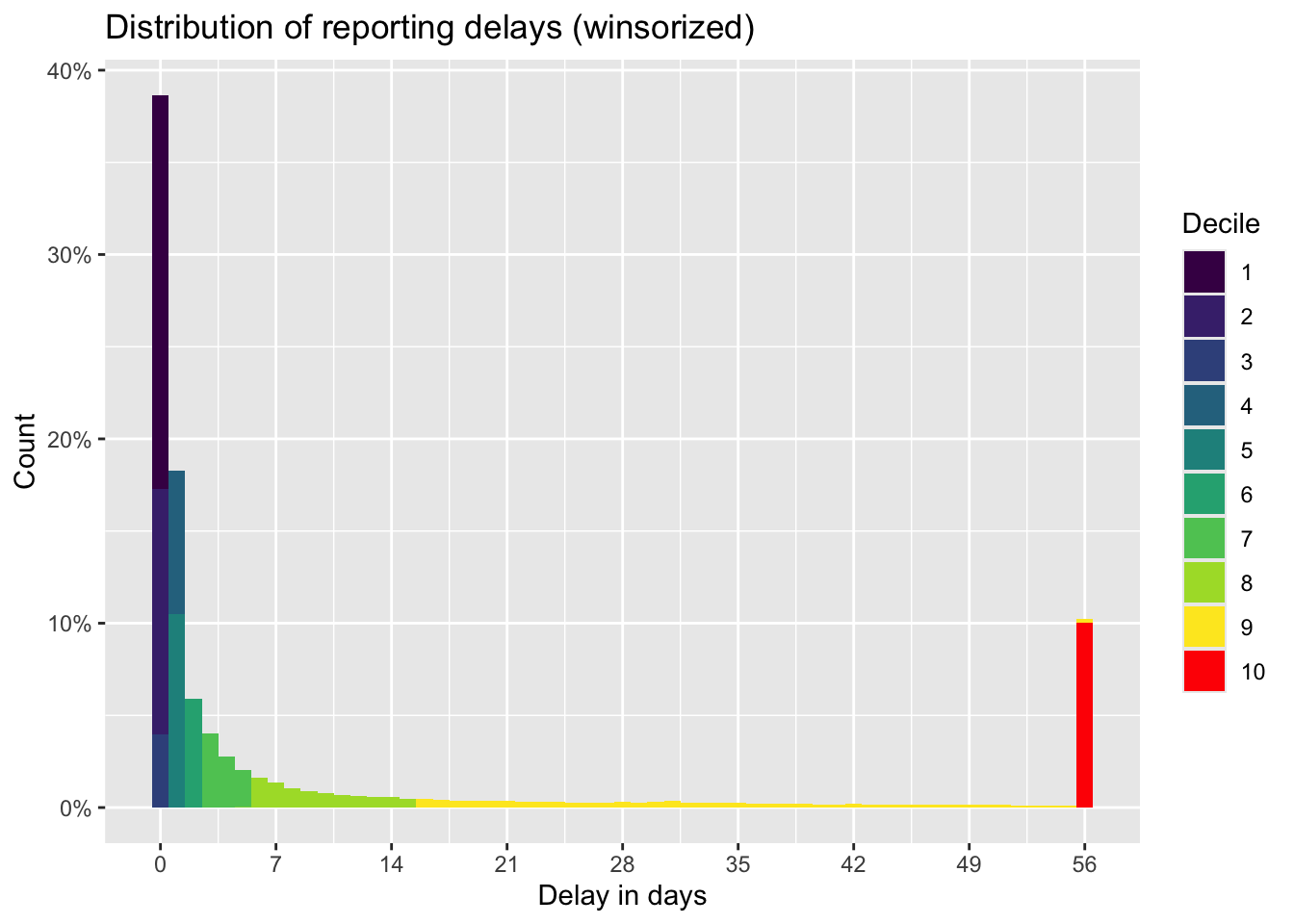
I do two things: Take log(delay+1) to dampen the impact of outliers
data %>% count(delay_hours)# A tibble: 2,995 × 2
delay_hours n
<dbl> <int>
1 22059. 1
2 22276. 1
3 22417. 1
4 22448. 1
5 22634. 1
6 22694. 1
7 22708. 1
8 22820. 1
9 22866. 1
10 22974. 1
# ℹ 2,985 more rowsdata <- data %>%
mutate(log_delay_full_days = log(delay_full_days + 1),
log_delay_hours = log(delay_hours))And exclude the top decile of delays i.e. reported about more than two months (56 days) after the crime, and sometimes many years after. In those cases, temperature on the day is probably not a big driver. Those very long delays likely represents special cases where the reporting dynamics are different from typical cases, especially given that we are interested in the effects of temperature on the decision to report. Long delays (e.g. several months or years) might reflect administrative issues, legal complexities, or other factors unrelated to temperature.
Estimations
I estimate log(delay) as a function of temperature, controlling for other factors, varying the sample I include.
# Fit the model using fixest
reg_delay_d_full <- data %>%
  filter(delito_lumped == "Domestic violence") %>%
  feols(log_delay_full_days ~ tmean |
          prec_quintile + rh_quintile + wsp_quintile + hour_hecho +
          ageb + year^month + day_of_week + day_of_year,
        cluster = ~ ageb)

reg_delay_d_90 <- data %>%
  filter(delito_lumped == "Domestic violence",
         decile_delay_full_days <= 9) %>%
  feols(log_delay_full_days ~ tmean |
          prec_quintile + rh_quintile + wsp_quintile + hour_hecho +
          ageb + year^month + day_of_week + day_of_year,
        cluster = ~ ageb)

reg_delay_d_80 <- data %>%
  filter(delito_lumped == "Domestic violence",
         decile_delay_full_days <= 8) %>%
  feols(log_delay_full_days ~ tmean |
          prec_quintile + rh_quintile + wsp_quintile + hour_hecho +
          ageb + year^month + day_of_week + day_of_year,
        cluster = ~ ageb)

etable(reg_delay_d_full, reg_delay_d_90, reg_delay_d_80,
       view = T)
reg_delay_d_full reg_delay_d_90 reg_delay_d_80
Dependent Var.: log_delay_full_days log_delay_full_days log_delay_full_days
tmean -0.0137** (0.0052) -0.0068. (0.0040) -0.0025 (0.0029)
Fixed-Effects: ------------------- ------------------- -------------------
prec_quintile Yes Yes Yes
rh_quintile Yes Yes Yes
wsp_quintile Yes Yes Yes
hour_hecho Yes Yes Yes
ageb Yes Yes Yes
year-month Yes Yes Yes
day_of_week Yes Yes Yes
day_of_year Yes Yes Yes
_______________ ___________________ ___________________ ___________________
S.E.: Clustered by: ageb by: ageb by: ageb
Observations 80,921 75,598 68,129
R2 0.09561 0.07901 0.08921
Within R2 9.91e-5 4.25e-5 1.18e-5
---
Signif. codes: 0 '***' 0.001 '**' 0.01 '*' 0.05 '.' 0.1 ' ' 1The positive association between temperature and faster reporting is driven largely by longer delays. Once these longer delays are removed, the effect of temperature diminishes or disappears. This suggests that while temperature does influence reporting behavior, its impact is primarily seen in cases with longer reporting delays. This supports the idea of a reporting bias: hotter weather likely accelerates reporting for cases that would have otherwise been delayed, but for shorter delays, temperature plays a much smaller role.
Short vs long delays: interactions
Does temperature affect reporting behavior differently across delay types? ie are shorter delays more sensitive to temperature than longer delays?
First, categorize the delays in different categories:
data %>% count(delay_full_days)# A tibble: 2,601 × 2
delay_full_days n
<dbl> <int>
1 0 343013
2 1 162285
3 2 52433
4 3 35744
5 4 24484
6 5 18102
7 6 14605
8 7 12106
9 8 9144
10 9 7747
# ℹ 2,591 more rowsdata <- data %>%
arrange(delay_full_days) %>%
mutate(delay_category_full_days = case_when(
delay_full_days %in% 0:1 ~ "[0-1]",
delay_full_days %in% 2:7 ~ "[2-7]",
delay_full_days %in% 7:14 ~ "[7-14]",
delay_full_days %in% 15:56 ~ "[15-56]",
delay_full_days > 56 ~ "(56)"),
delay_category_full_days = as_factor(delay_category_full_days))
data %>% count(delay_category_full_days) %>%
filter(!is.na(delay_category_full_days)) %>%
mutate(freq = n/sum(n))# A tibble: 5 × 3
delay_category_full_days n freq
<fct> <int> <dbl>
1 [0-1] 505298 0.569
2 [2-7] 157474 0.177
3 [7-14] 45382 0.0511
4 [15-56] 89790 0.101
5 (56) 89629 0.101 Now run the regressions:
reg_interacted_days <- data %>%
  filter(delito_lumped == "Domestic violence") %>%
  feols(log_delay_full_days ~ i(delay_category_full_days, temp) |
          prec_quintile + rh_quintile + wsp_quintile + hour_hecho +
          ageb + year^month + day_of_week + day_of_year,
        cluster = ~ ageb)

etable(reg_interacted_days, view = T)
reg_interacted_days
Dependent Var.: log_delay_full_days
temp x delay_category_full_days = [0-1] -0.0576*** (0.0017)
temp x delay_category_full_days = [2-7] 0.0038* (0.0017)
temp x delay_category_full_days = [7-14] 0.0582*** (0.0017)
temp x delay_category_full_days = [15-56] 0.1094*** (0.0017)
temp x delay_category_full_days = (56) 0.2023*** (0.0018)
Fixed-Effects: -------------------
prec_quintile Yes
rh_quintile Yes
wsp_quintile Yes
hour_hecho Yes
ageb Yes
year-month Yes
day_of_week Yes
day_of_year Yes
________________________________________ ___________________
S.E.: Clustered by: ageb
Observations 80,921
R2 0.91886
Within R2 0.91029
---
Signif. codes: 0 '***' 0.001 '**' 0.01 '*' 0.05 '.' 0.1 ' ' 1iplot(reg_interacted_days)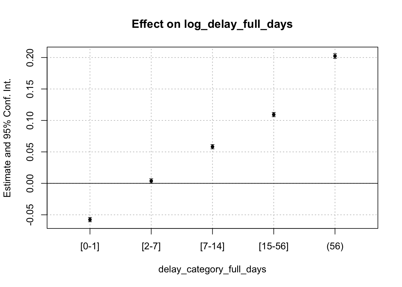
This analysis shows that while temperature accelerates immediate reporting, it also significantly slows down long-term reporting (beyond a couple of days). This is a problem…
Weather on the Day of Reporting
At the incident level, we have precise information on when the crime was reported. By looking at temperature on the report day, I directly test whether temperature affects when victims report crimes (i.e., whether victims are more likely to report crimes on hot days). This helps to isolate reporting behavior from the actual incidence of the crime.
If the report-day temperature significantly affects the length of the reporting delay, this suggests that temperature-driven reporting bias could be a factor.
reg_delay_d_extra_weather_full <- data %>%
  filter(delito_lumped == "Domestic violence") %>%
  feols(log_delay_full_days ~ tmean + tmean_report_day +
          prec + rh + wsp +
          prec_report_day + rh_report_day + wsp_report_day |
          hour_hecho +
          ageb + year^month + day_of_week + day_of_year,
        cluster = ~ ageb)

etable(reg_delay_d_extra_weather_full)
reg_delay_d_extra..
Dependent Var.: log_delay_full_days
tmean -0.0329*** (0.0067)
tmean_report_day 0.0357*** (0.0069)
prec -0.0006 (0.0021)
rh -0.0030** (0.0011)
wsp -0.0357* (0.0169)
prec_report_day 0.0096*** (0.0018)
rh_report_day 0.0065*** (0.0011)
wsp_report_day 0.0946*** (0.0154)
Fixed-Effects: -------------------
hour_hecho Yes
ageb Yes
year-month Yes
day_of_week Yes
day_of_year Yes
________________ ___________________
S.E.: Clustered by: ageb
Observations 80,919
R2 0.09781
Within R2 0.00285
---
Signif. codes: 0 '***' 0.001 '**' 0.01 '*' 0.05 '.' 0.1 ' ' 1Problem: report-day temperature is significant. This could indicate that temperature affects reporting behavior, contributing to the total effect seen in the main analysis.
The results show that temperatures on both the day of the crime and the day of reporting influence reporting delays, with hot weather on the crime day accelerating reporting and hot weather on the report day delaying it.
Fix 1: Look at different types of crime
To try and isolate the true effect of temperature on crime incidence, I try to compare DV crimes with another type of crime that is less affected by reporting behavior (e.g., property crimes like theft, where reporting is more consistent regardless of temperature).
If temperature was to only affect the reporting of DV and not other crimes, this would point to the likelihood of a reporting bias. However, I found that temperature affects all types of crimes similarly (be it when measured in full days, or in hours). This is good news, as it shows that temperature has a direct effect on crime occurrence, not just reporting. Maybe it is simply the judicial system that is affected by temperatures?
reg_types_days <- data %>%
  filter(delito_lumped != "Suicides") %>%
  filter(delito_lumped != "Feminicide") %>%
  feols(log_delay_full_days ~ tmean |
          prec_quintile + rh_quintile + wsp_quintile + hour_hecho +
          ageb + year^month + day_of_week + day_of_year,
        cluster = ~ ageb,
        split = ~ delito_lumped)

etable(reg_types_days, view = T)
reg_types_days.1 reg_types_days.2
Sample (delito_lumped) Domestic violence Drugs related
Dependent Var.: log_delay_full_days log_delay_full_days
tmean -0.0137** (0.0052) -0.0064 (0.0082)
Fixed-Effects: ------------------- -------------------
prec_quintile Yes Yes
rh_quintile Yes Yes
wsp_quintile Yes Yes
hour_hecho Yes Yes
ageb Yes Yes
year-month Yes Yes
day_of_week Yes Yes
day_of_year Yes Yes
______________________ ___________________ ___________________
S.E.: Clustered by: ageb by: ageb
Observations 80,921 16,009
R2 0.09561 0.23807
Within R2 9.91e-5 9.03e-5
reg_types_days.3 reg_types_days.4
Sample (delito_lumped) Fraud Homicide
Dependent Var.: log_delay_full_days log_delay_full_days
tmean -0.0083 (0.0093) -0.0042 (0.0115)
Fixed-Effects: ------------------- -------------------
prec_quintile Yes Yes
rh_quintile Yes Yes
wsp_quintile Yes Yes
hour_hecho Yes Yes
ageb Yes Yes
year-month Yes Yes
day_of_week Yes Yes
day_of_year Yes Yes
______________________ ___________________ ___________________
S.E.: Clustered by: ageb by: ageb
Observations 51,012 6,801
R2 0.27571 0.39571
Within R2 1.82e-5 3.89e-5
reg_types_days.5 reg_types_days.6
Sample (delito_lumped) Other Rapes
Dependent Var.: log_delay_full_days log_delay_full_days
tmean -0.0039 (0.0034) 0.0069 (0.0629)
Fixed-Effects: ------------------- -------------------
prec_quintile Yes Yes
rh_quintile Yes Yes
wsp_quintile Yes Yes
hour_hecho Yes Yes
ageb Yes Yes
year-month Yes Yes
day_of_week Yes Yes
day_of_year Yes Yes
______________________ ___________________ ___________________
S.E.: Clustered by: ageb by: ageb
Observations 237,565 3,594
R2 0.18090 0.65488
Within R2 5.31e-6 8.22e-6
reg_types_days.7 reg_types_days.8
Sample (delito_lumped) Sexual crimes Theft
Dependent Var.: log_delay_full_days log_delay_full_days
tmean -0.0015 (0.0224) -0.0012 (0.0019)
Fixed-Effects: ------------------- -------------------
prec_quintile Yes Yes
rh_quintile Yes Yes
wsp_quintile Yes Yes
hour_hecho Yes Yes
ageb Yes Yes
year-month Yes Yes
day_of_week Yes Yes
day_of_year Yes Yes
______________________ ___________________ ___________________
S.E.: Clustered by: ageb by: ageb
Observations 10,975 419,686
R2 0.38586 0.06108
Within R2 5.81e-7 9.9e-7
reg_types_days.9 reg_types_days.10
Sample (delito_lumped) Threats Trust abuse
Dependent Var.: log_delay_full_days log_delay_full_days
tmean -0.0107 (0.0071) 0.0048 (0.0161)
Fixed-Effects: ------------------- -------------------
prec_quintile Yes Yes
rh_quintile Yes Yes
wsp_quintile Yes Yes
hour_hecho Yes Yes
ageb Yes Yes
year-month Yes Yes
day_of_week Yes Yes
day_of_year Yes Yes
______________________ ___________________ ___________________
S.E.: Clustered by: ageb by: ageb
Observations 44,014 15,046
R2 0.14137 0.32377
Within R2 5.83e-5 7.23e-6
---
Signif. codes: 0 '***' 0.001 '**' 0.01 '*' 0.05 '.' 0.1 ' ' 1# for full days
data %>% count(delito_lumped)# A tibble: 12 × 2
delito_lumped n
<chr> <int>
1 Domestic violence 80921
2 Drugs related 16009
3 Feminicide 204
4 Fraud 51021
5 Homicide 6803
6 Other 237569
7 Rapes 3594
8 Sexual crimes 10977
9 Suicides 1724
10 Theft 419689
11 Threats 44015
12 Trust abuse 15047reg_types_days_interacted <- data %>%
filter(delito_lumped != "Suicides") %>%
filter(delito_lumped != "Feminicide") %>%
feols(log_delay_full_days ~ i(delay_category_full_days, tmean) |
prec_quintile + rh_quintile + wsp_quintile + hour_hecho +
ageb + year^month + day_of_week + day_of_year,
cluster = ~ ageb,
split = ~ delito_lumped)
# etable(reg_types_days, view = T)
# etable(reg_types_days[1:5], view = T)
# etable(reg_types_days[6:10], view = T)
# Plot them all
coeftable(reg_types_days_interacted) %>%
as_tibble() %>%
mutate(ci_lo = Estimate - 1.96*`Std. Error`,
ci_hi = Estimate + 1.96*`Std. Error`) %>%
mutate(coefficient = as_factor(str_extract(coefficient, "(?<=::).*?(?=:)"))) %>%
ggplot(aes(x = Estimate, y = coefficient, color = sample)) +
geom_pointrange(aes(xmin = ci_lo, xmax = ci_hi), fatten = 2) +
#add vline at 0
geom_vline(xintercept = 0, linetype = "dashed") +
scale_y_discrete(guide = guide_axis(angle = 45)) +
coord_flip() +
facet_wrap(~sample) +
theme(legend.position = "none") +
labs(title = "Effect of temperature on reporting delays by crime type",
subtitle = "Full days data, but also full period",
x = NULL,
y = NULL)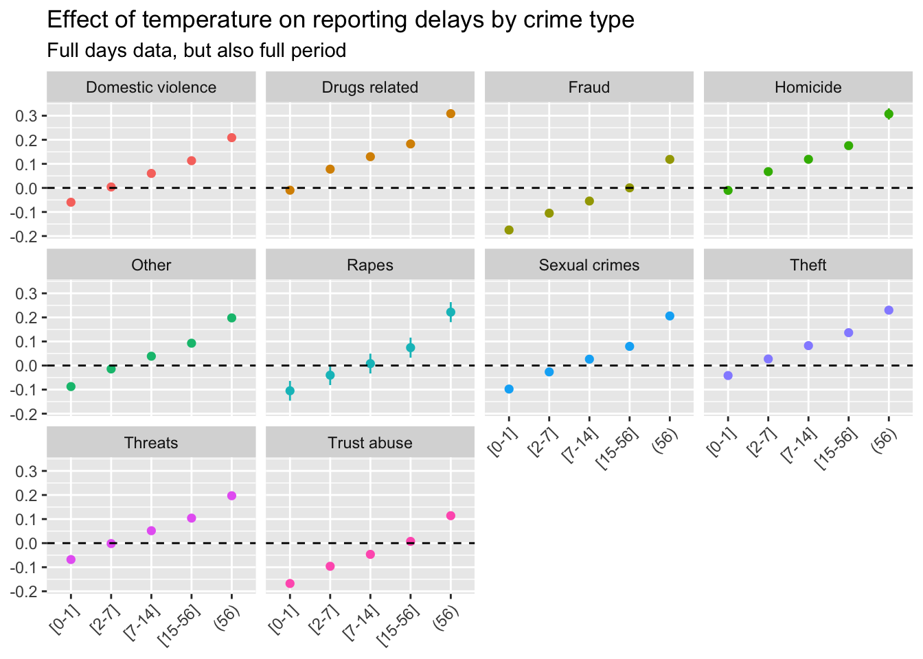
Fix 2: Use Reporting Time Categories as a Test for Reporting Bias
Another way to test for reporting bias is to examine different time categories of reporting (e.g., within the same day, 1-7 days, more than 7 days) to see if the temperature effect on DV incidents is different for different reporting delays.
For that purpose, I need to count the number of crimes per day per neighborhood per category of crime. IE the level is not done at the crime level anymore, but at the day per neighborhood level, like in the main analysis. I also do count model instead of log-linear and estimate with PPML. I did this in a previous file.
final_data <-
  read_rds(here("..", "output",
                "data_reports.rds")) %>%
  filter(year %in% 2016:2019)

final_data %>%
  select(contains("reports_dv_delay")) %>%
  names()

#weird names fuck up the fixest estimations
final_data <- final_data %>%
  rename_with(~ str_replace_all(., "[\\[\\]()]", "")) %>%  # Remove brackets and parentheses
  rename_with(~ str_replace_all(., "-", "_"))              # Replace dashes with underscores
Looking at hours
Run the regressions looking at hours.
reg_delays_hours <-
  fepois(c(reports_dv_delay_hours_0_6,
           reports_dv_delay_hours_6_24,
           reports_dv_delay_hours_24_48,
           reports_dv_delay_hours_48_168,
           reports_dv_delay_hours_168_) ~ tmean |
           ageb + year^month + day_of_week + day_of_year +
           prec_quintile + rh_quintile + wsp_quintile,
         cluster = ~ ageb,
         data = final_data)

etable(reg_delays_hours, view = T)
The coefficients for temp tell us how a 1°C increase in temperature affects the number of DV incidents reported in each time category, after controlling for other variables.
Across diff specs, not very significant effects, still some. - Higher temperatures might slightly increase the number of DV crimes reported within 6-24 hours. - Higher temperatures are associated with a significant increase in DV crimes reported after 2-7 days.
This means that temperature has a stronger effect on delayed reporting (2-7 days) than on immediate reporting (within 0-6 hours). This could indicate that while temperature might influence the overall incidence of domestic violence, it also seems to play a role in delaying the reporting process for some incidents.
The good news
If the temperature effect were large and significant for immediate reports, it would have been more difficult to argue that the increase in reported DV incidents wasn’t driven by reporting bias. The fact that temperature has limited impact on immediate reports suggests that the observed rise in domestic violence during hotter days is likely not just due to faster reporting, but rather indicates a real increase in crime incidence.
The bad news
For delayed reporting (48-168 hours), the effect of temperature is positive and statistically significant, indicating that higher temperatures significantly increase the number of crimes reported with a delay. This could be an indication of reporting bias for crimes that aren’t reported immediately.
Looking at full days
Coarser measure, but more data
reg_delays_days <-
  fepois(c(reports_dv_delay_days_0,
           reports_dv_delay_days_1,
           reports_dv_delay_days_2_7,
           reports_dv_delay_days_7_14,
           reports_dv_delay_days_14_) ~ tmean |
           ageb + year^month + day_of_week + day_of_year +
           prec_quintile + rh_quintile + wsp_quintile,
         cluster = ~ ageb,
         data = final_data)

etable(reg_delays_days, view = T)
I find that higher temperatures are associated with a significant increase in DV crimes, positive, significant, and consistent across categories (about 2,5%) (excpet for more than two weeks delay).
Reporting Bias Concerns:
Good News: The significant temperature effect on same-day and next-day reporting strengthens the argument that higher temperatures lead to quicker reporting and suggest that reporting bias is less likely to be driving your main findings of increased DV incidence.
Some Concerns: The significant positive effect for delays up to 14 days could indicate that temperature also encourages delayed reports, meaning that some part of the increase in reported incidents could still be due to changes in reporting behavior over time, not just crime incidence.
Overall, the effect is not concentrated in same-day reports, this could indicate that reporting bias does not play a significant role.
Alternatively, if the effect persists across all reporting categories, it suggests that temperature is influencing the actual incidence of DV, not just the speed of reporting.
How do i do this?
Count the number of crimes by reporting time category in the further files. Run the regressions in here, and clean up this file a bit. Then call it quits.
Next steps
Exclude late reports
Should I just run the main regressions but kicking out the cases for which delay is more than 2 weeks? those could be the ones measured with errors or sth. I can just add all reports_dv_delay_days_0 reports_dv_delay_days_1 reports_dv_delay_days_2_7 reports_dv_delay_days_7_14 to create a new measure of reports_dv_censored. no need to go back to counting.