AGEBs and their characteristics

Note

In this file, I process the borders of statistical units of Mexico City, the AGEBs.

I then import several datasets on AGEB characteristics, such as population, poverty, social deprivation, etc.

I save two files:

• ageb_poligonos.geojson: the borders of the AGEBs, a geographical file
• ageb_attributes.rds: a tibble with all the characteristics of the AGEBs

Mexico is organised in about 2000 neighborhoods (colonias). There are no official and stable definitions for these neighborhoods.

So, I will use another administrative unit to count the calls, the AGEB (Área geoestadística Básica), which is a geographical area defined by INEGI (statistical institute). There are about 2500 AGEBs in Mexico City. Most neighborhood characteristics are distributed at the AGEB level, which is also the level of the census etc.

Note that there is no direct correspondance between AGEB and colonias. In the next file, I look at colonias which is needed to locate the calls.

1 AGEBs gegraphical borders

# AGEB BORDERS
# 09a.shp is the level we want, the rest is other levels
poligonos <- 
  read_sf(here("..", "raw_data", "1_ageb",
               "marco_geoestadistico", "conjunto_de_datos",
               "09a.shp"),
          quiet = TRUE) %>%
  st_transform(4326) %>% 
  st_make_valid() %>% 
  select(ageb = CVEGEO)

We have the physical borders of the 2431 AGEBs, those from INEGI’s Marco Geoestadístico. Censo de Población y Vivienda 2020

poligonos %>% 
  ggplot() +
  geom_sf() +
  annotation_scale(location = "br", style = "ticks") +
  theme_minimal()

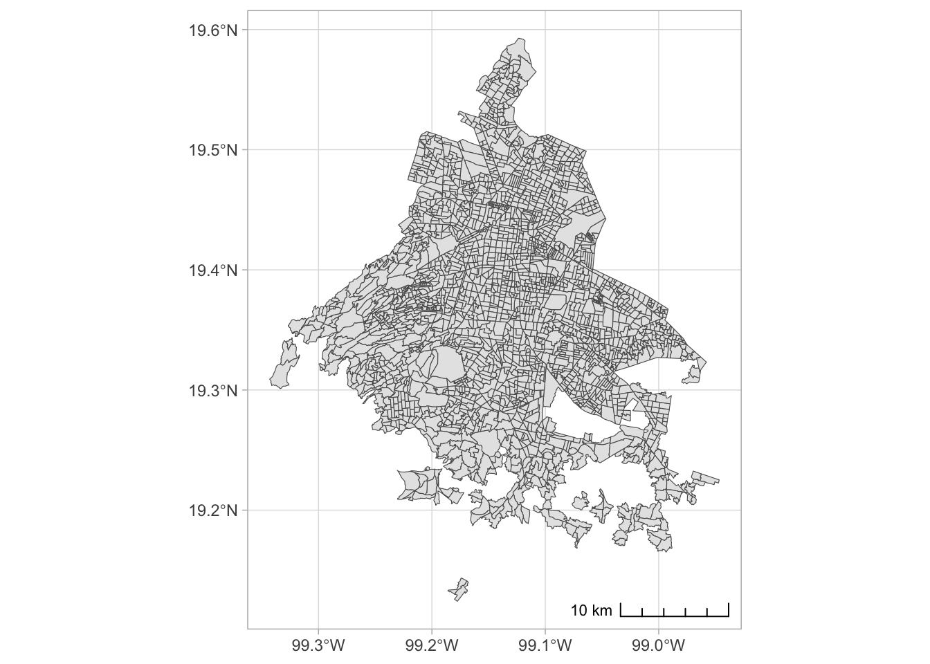
2 AGEBs characteristics

Import the different datasets

I have several sources of data on AGEB characteristics (sources, description, and data dictionary in their respective folders).

1. CPV: census poblacion y vivienda 2020 (INEGI)
2. GRS: grado rezago social 2020 (CONEVAL)
3. IMU: indice de marginacion urbana 202O (CONAPO)
4. IDS: indice de desarrollo social 2020 (EVALUA)
5. Pobreza: Pobreza urbana 2020 (CONEVAL)
6. Income: ingresos trimestriales 2014 (IPDP)

(ENIGH is not really useful, since it is at the municipality level – only 16 for the whole of CMDX)

I import them all, select the relevant variables and merge them into a single dataset.

# CPV
censo <- 
  read_csv(here("..", "raw_data", "1_ageb",
               "cpv2020", "conjunto_de_datos",
               "conjunto_de_datos_ageb_urbana_09_cpv2020.csv")) %>% 
  rename_with(tolower)
censo %>% count(nom_loc) %>% 
  filter(str_detect(nom_loc, "Total")) %>% 
  kable()
# the data is at the city block level, too precise
# we want to use the AGEB aggregates
censo  <- censo %>% 
  filter(nom_loc == "Total AGEB urbana") 
sum(censo$pobtot)
# create ageb
censo <- censo %>% 
  mutate(ageb = paste0(entidad, mun, loc, ageb)) %>% 
  select(ageb, nom_ent, nom_mun, pobtot:vph_sintic)

# there are tons of variables, heres the dicitionary
censo_dicc <- 
    read_csv(here("..", "raw_data", "1_ageb",
               "cpv2020", "diccionario_de_datos",
               "diccionario_datos_ageb_urbana_09_cpv2020.csv"),
             skip = 3) %>% 
  rename_with(tolower) %>% 
  relocate(mnemónico, indicador, descripción) 

# GRS
grs <- 
  read_excel(here("..", "raw_data", "1_ageb",
               "grs_coneval", "GRS_AGEB_urbana_2020.xlsx"),
             range = "A4:AB61436",
             col_names = FALSE) %>% 
  rename_with(tolower)
# rename
colnames(grs) <- ifelse(is.na(grs[2, ]), grs[1, ], grs[2, ])
grs <- grs %>% filter(`Entidad\r\nfederativa` == "Ciudad de México")

grs <- grs %>% 
  select(ageb = `Clave de la AGEB`,
         pobtot = `Población total`,
         grs = `Grado de Rezago Social`,
         vivtot = `Viviendas particulares habitadas con caracteristicas`,
         `Población de 15 años o más analfabeta`:`Viviendas que no disponen de internet`)
  
# IMU
imu <- 
  read_excel(here("..", "raw_data", "1_ageb",
               "imu_2020", "IMU_2020.xls"),
             skip = 0, col_names = FALSE)
imu_dicc <- imu %>% 
  slice(4,6) %>% 
  t()

imu <- imu %>% 
  rename_with(~ as.character(imu[6, ])) %>% 
  rename_with(tolower) %>% 
  filter(nom_ent == "Ciudad de México") %>% 
  select(ageb = cve_ageb, pob_tot:imn_2020)

ids <- 
  read_sf(here("..", "raw_data", "1_ageb",
               "ids_ageb", "ids_ageb_cdmx.shp"),
          quiet = TRUE) %>% 
  st_drop_geometry() %>% 
  select(ageb = cvegeo, pobtotal:ids) %>% 
  as_tibble()

ids_dicc <- 
  read_excel(here("..", "raw_data", "1_ageb", "ids_ageb", "diccionario_ageb.xlsx")) %>% 
  mutate(
    weight = case_when(
      Etiqueta == "ids_cassi" ~ 0.1415,
      Etiqueta == "ids_casi" ~ 0.1415,
      Etiqueta == "ids_ccevj" ~ 0.328,
      Etiqueta == "ids_rei" ~ 0.236,
      Etiqueta == "ids_cbdj" ~ 0.058,
      Etiqueta == "ids_caej" ~ 0.028,
      Etiqueta == "ids_csj" ~ 0.037,
      Etiqueta == "ids_ctelj" ~ 0.030,
      TRUE ~ NA_real_
    )
  ) %>% filter(!is.na(weight)) %>% arrange(desc(weight))

pobreza <- readxl::read_excel(
  here("..", "raw_data", "1_ageb", "pobreza_ageb_coneval",
       "Base de datos de pobreza AGEB segun entidad federativa 2015.xlsx"),
  sheet = "Ciudad de México",
  range = "B8:H2439",
  col_names = FALSE) %>%
  select(ageb = ...5, pobreza = ...6, pobrezaex = ...7) %>% 
  arrange(as.numeric(str_sub(pobreza, 2, 3)),
          as.numeric(str_sub(pobrezaex, 2, 3))) %>%
  mutate(pobreza = as_factor(pobreza), 
         pobrezaex = as_factor(pobrezaex))

income <-
  read_sf(here("..", "raw_data", "1_ageb",
               "ingresos_trimestrales",
               "ingresos_trimestrales.shp"),
          quiet = TRUE) %>% 
  st_drop_geometry() %>% 
  mutate(income = na_if(IngMon_14, 0)) %>% 
  select(ageb = CVEGEO, income)

#Income in hex, more recent (2918), but much less detailed
# categories (1-25k-50k-100k-150k- more)
# AND hex, not AGEB

hex <-
  read_sf(here("..", "raw_data", "1_ageb",
               "ingresos_trimestrales", "hex_ingresos_2018",
               "hex_ingresos_unidos.shp")) %>% 
  st_transform(crs = 4326) %>% 
  mutate(order = sub(" .*", "", r_ingreso),
         order = as.numeric(gsub(",", "", order))) %>% 
  arrange(order) %>% 
  mutate(r_ingreso = as_factor(r_ingreso))

hex %>% 
  ggplot() +
  geom_sf(aes(fill = r_ingreso),
          color = gray(.2),
          alpha = .7) +
  annotation_scale(location = "br", style = "ticks") +
  scale_fill_brewer(palette = 4) +
  theme_minimal()

Compare unit of analysis and uniformise

Data is recorded at AGEB level in all datasets but there are some slight variations. It’s very minimal. I uniformise everything.

# List of AGEBs in each dataset
agebs <- list(
  poligonos = poligonos %>% st_drop_geometry() %>% select(ageb) %>% distinct() %>% as_tibble(),
  censo = censo %>% distinct(ageb),
  grs = grs %>% distinct(ageb),
  ids = ids %>% distinct(ageb),
  imu = imu %>% distinct(ageb),
  income = income %>% distinct(ageb),
  pobreza = pobreza %>% distinct(ageb)
)

all_agebs <- bind_rows(agebs) %>% distinct()
# Create a presence matrix dynamically with dataset names
agebs <- all_agebs %>% 
  mutate(across(everything(), as.character)) %>%
  bind_cols(
    map_dfc(names(agebs), ~ as.integer(all_agebs$ageb %in% pull(agebs[[.x]], ageb))) %>%
      set_names(paste0("in_", names(agebs)))  # Keep original dataset names
  ) %>%
  as_tibble() %>% 
  mutate(total_present = rowSums(select(., starts_with("in_"))))

#Count number of missing AGEBs per dataset (sum of 0s in each column)
agebs %>%
  summarise(across(starts_with("in_"), ~ sum(. == 0)))

# Reference: AGEBs in poligonos
poligonos_agebs <- poligonos %>% pull(ageb)

# Count missing AGEBs per dataset (AGEBs in poligonos but missing elsewhere)
agebs %>%
  filter(ageb %in% poligonos_agebs) %>%
  summarise(across(starts_with("in_"), ~ sum(. == 0)))

# Count extra AGEBs per dataset (AGEBs not in poligonos but present elsewhere)
agebs %>%
  filter(!ageb %in% poligonos_agebs) %>%
  summarise(across(starts_with("in_"), ~ sum(. == 1)))

Filter all datasets to only include AGEBs that are in the official borders.

censo <- 
  censo %>% filter(ageb %in% poligonos_agebs)
grs <- 
  grs %>% filter(ageb %in% poligonos_agebs)
ids <- 
  ids %>% filter(ageb %in% poligonos_agebs)
imu <- 
  imu %>% filter(ageb %in% poligonos_agebs)
income <- 
  income %>% filter(ageb %in% poligonos_agebs)
pobreza <- 
  pobreza %>% filter(ageb %in% poligonos_agebs)

Look at the variables we have

We have a look at the different characteristics of the AGEBs in each dataset.

Censo

Rawest data, from 2020 Censo de Població, y Vivienda. Contains population disagregated by many aspects. Also contains number of households with piso de tierra, number of rooms…

censo_dicc %>% 
  select(mnemónico, indicador) %>% 
  datatable()

Show 102550100 entries

Search:

	mnemónico	indicador
1	ENTIDAD	Clave de entidad federativa
2	NOM_ENT	Entidad federativa
3	MUN	Clave de municipio o demarcación territorial
4	NOM_MUN	Municipio o demarcación territorial
5	LOC	Clave de localidad
6	NOM_LOC	Localidad
7	AGEB	Clave del AGEB
8	MZA	Clave de manzana
9	POBTOT	Población total
10	POBFEM	Población femenina

Showing 1 to 10 of 230 entries

Previous12345…23Next

# POBTOT Población total
# POB_AFRO Población que se considera afromexicana o afrodescendiente
# PEA Población de 12 años y más económicamente activa
# VIVPARH_CV Total de viviendas particulares habitadas con características

# VPH_PISODT Viviendas particulares habitadas con piso de material diferente de tierra
# VPH_PISOTI Viviendas particulares habitadas con piso de tierra
# .... way more VPH_sth, like number of rooms, with or without electricity,
# water, car, internet, etc...
# VPH_SINTIC Viviendas particulares habitadas sin tecnologías de la información y de la comunicación (TIC)

censo %>% select(ageb, pobtot, pob_afro, pea, vivparh_cv,
                 starts_with("vph_")) %>% head() %>% kable()

ageb	pobtot	pob_afro	pea	vivparh_cv	vph_pisodt	vph_pisoti	vph_1dor	vph_2ymasd	vph_1cuart	vph_2cuart	vph_3ymasc	vph_c_elec	vph_s_elec	vph_aguadv	vph_aeasp	vph_aguafv	vph_tinaco	vph_cister	vph_excsa	vph_letr	vph_drenaj	vph_nodren	vph_c_serv	vph_ndeaed	vph_dsadma	vph_ndacmm	vph_snbien	vph_refri	vph_lavad	vph_hmicro	vph_autom	vph_moto	vph_bici	vph_radio	vph_tv	vph_pc	vph_telef	vph_cel	vph_inter	vph_stvp	vph_spmvpi	vph_cvj	vph_sinrtv	vph_sinltc	vph_sincint	vph_sintic
0900200010010	3183	98	1582	865	864	*	81	784	*	11	852	865	0	865	865	0	720	26	865	0	865	0	865	0	865	376	0	858	824	669	479	47	177	717	850	532	741	772	692	313	221	145	8	14	148	5
0900200010025	5593	142	2854	1759	1759	0	172	1587	0	25	1734	1759	0	1759	1739	0	375	370	1759	0	1759	0	1759	0	1759	1216	*	1730	1614	1246	515	61	243	1286	1707	930	1373	1510	1203	478	349	238	28	68	393	14
090020001003A	4235	13	2152	1184	1184	0	175	1009	*	9	1174	1184	0	1183	1183	*	472	17	1184	0	1184	0	1183	0	1184	742	*	1162	1070	816	422	35	215	970	1168	641	965	1049	878	361	339	247	5	12	250	*
0900200010044	4768	123	2432	1389	1388	0	160	1229	*	11	1376	1389	0	1389	1376	0	672	65	1389	0	1389	0	1389	0	1389	782	0	1371	1286	1019	579	70	245	1111	1365	845	1124	1237	1076	481	452	294	10	17	254	*
0900200010097	2176	12	1091	596	596	0	23	573	*	8	587	596	0	596	596	0	470	30	596	0	596	0	596	0	596	299	0	592	562	470	289	25	48	482	591	399	517	562	507	276	260	153	4	3	70	0
090020001010A	3346	29	1635	910	910	0	71	839	*	*	906	910	0	910	909	0	689	43	910	0	910	0	910	0	909	452	0	903	859	700	446	40	153	755	903	646	815	824	768	344	389	213	*	4	112	0

Grado de Rezago Social

Grado de Rezago Social (GRS) is a measure of social deprivation, published by CONEVAL.

They compute 17 indicators:

• some shares of the population that doesnt attend school,
• share of houses with piso de tierra, etc…

They’re the same variables as in censo, but as shares.

#Grado de Rezago Social
names(grs) %>% kable()

x
ageb
pobtot
grs
vivtot
Población de 15 años o más analfabeta
Población de 6 a 14 años que no asiste a la escuela
Población de 15 a 24 años que no asiste a la escuela
Población de 15 años o más con educación básica incompleta
Población sin derechohabiencia a servicios de salud
Viviendas con hacinamiento
Viviendas que no disponen de agua entubada de la red pública
Viviendas que no disponen de excusado o sanitario
Viviendas que no disponen de drenaje
Viviendas que no disponen de energía eléctrica
Viviendas con piso de tierra
Viviendas que no disponen de lavadora
Viviendas que no disponen de refrigerador
Viviendas que no disponen de teléfono fijo
Viviendas que no disponen de celular
Viviendas que no disponen de computadora (computadora, laptop o tablet)
Viviendas que no disponen de internet

Then with these, using Análisis de Clases Latentes (LCA) it creates GRS, which is a measure of social deprivation, by categories only.

grs %>% count(grs) %>% kable()

grs	n
Alto	22
Bajo	1234
Medio	200
Muy alto	6
Muy bajo	948

Not very useful…

Indice de Desarrollo Social

Published by EVALUA, Consejo de Evalución de la Ciudad de Mexico. Based on variables from the Encuesta Nacional de Ingresos y Gastos de los Hogares (ENIGH), it computes 8 indices of social development at AGEB level.

1. IDS de Vivienda : Carencia en la calidad y espacios de la vivienda;
2. IDS de Educación : Rezago educativo por persona;
3. IDS de Seguridad social : Carencia en el Acceso a los Servicios de Seguridad Social por persona:
4. IDS de Salud : Carencia en el acceso a servicios de salud por persona;
5. IDS de Bienes durables : Carencia de Bienes Durables;
6. IDS de Adec. sanitaria : Carencia de servicios sanitarios (agua y drenaje);
7. IDS de Telecomunicaciones : Carencia en el acceso a teléfono (fijo o celular) en el hogar;
8. IDS de Adec. energética : Carencia en adecuación Energética

Then with all those indices, weighting them, it computes an aggregate, ids.

CONEVAL also computes the total number of people in poverty within each AGEB: pobres_tot (Población pobre por Necesidades Básicas Insatisfechas (NBI)). They define poverty using a multidimensional approach, considering both income and social deprivations. The poverty classification includes individuals who experience at least one of the following deprivations while having an income below the established poverty threshold.

The indices are all computed a bit differently; for example:

1. Vivienda is two dimensional: 1) calidad de los materiales de la construcción (Walls, roof, flooring) y 2) Disponibilidad de espacio en la vivienda (number of rooms, bedrooms, kitchen…) per person in the hh.
2. Bienes durables: nueve bienes durables que normativamente debería poseer un hogar (bicicleta, aparato para escuchar música, pantalla, ventilador, estufa, refrigerador, licuadora, plancha y lavadora).
3. Adec. sanitaria: tres indicadores: agua entubada, drenaje y excusado.
4. Adec energetica: La electricidad, así como el combustible para preparar o calentar alimentos

ids_dicc %>% kable()

Número	Etiqueta	Descripción	weight
9	ids_ccevj	IDS de Vivienda	0.3280
14	ids_rei	IDS de Educación	0.2360
15	ids_cassi	IDS de Seguridad social	0.1415
16	ids_casi	IDS de Salud	0.1415
13	ids_cbdj	IDS de Bienes durables	0.0580
10	ids_csj	IDS de Adec. sanitaria	0.0370
12	ids_ctelj	IDS de Telecomunicaciones	0.0300
11	ids_caej	IDS de Adec. energética	0.0280

ids <- ids %>% 
  mutate(poverty_nbi = pobres_tot / pobtotal)

Indice de Marginacion Urbana

IMU is similar to IDS, focus on access to basic services and infrastructure. Identifies poor urban areas with infrastructure deficits.

These indicators are aggregated into a composite index using a weighted squared distances methodology

imu_dicc %>% kable()

…1	Clave geográfica	CVE_AGEB
…2	Clave de la entidad federativa	ENT
…3	Nombre de la entidad	NOM_ENT
…4	Clave del municipio	MUN
…5	Nombre del municipio	NOM_MUN
…6	Clave de la localidad	LOC
…7	Nombre de la localidad	NOM_LOC
…8	Clave de la AGEB	AGEB
…9	Población total	POB_TOT
…10	% Población de 6 a 14 años que no asiste a la escuela	P6A14NAE
…11	% Población de 15 años o más sin educación básica	SBASC
…12	% Población sin derechohabiencia a los servicios de salud	PSDSS
…13	% Ocupantes en viviendas particulares habitadas sin drenaje ni excusado	OVSDE
…14	% Ocupantes en viviendas particulares habitadas sin energía eléctrica	OVSEE
…15	% Ocupantes en viviendas particulares habitadas sin agua entubada	OVSAE
…16	% Ocupantes en viviendas particulares habitadas con piso de tierra	OVPT
…17	% Ocupantes en viviendas particulares habitadas con hacinamiento	OVHAC
…18	% Ocupantes en viviendas particulares habitadas sin refrigerador	OVSREF
…19	% Ocupantes en viviendas particulares habitadas sin internet	OVSINT
…20	% Ocupantes en viviendas particulares habitadas sin celular	OSCEL
…21	Índice de marginación, 2020	IM_2020
…22	Grado de marginación, 2020	GM_2020
…23	Índice de marginación normalizado, 2020	IMN_2020

Pobreza

Pobreza is a measure of poverty, based on the percentage of the population that is poor and extremely poor. Spatially imputated so not perfect, but crosses several data sources (see nota tecnica in source folder).

AGEBs are then classified into 5 poverty categories using statistical stratification. Missing for AGEB with 0 or only 1 household.

pobreza <- pobreza %>% 
  mutate(pobreza = na_if(pobreza, "Sin viviendas particulares habitadas"),
         pobreza = na_if(pobreza, "Una vivienda particular habitada"),
         pobrezaex = na_if(pobrezaex, "Sin viviendas particulares habitadas"),
         pobrezaex = na_if(pobrezaex, "Una vivienda particular habitada"))

pobreza %>% 
  count(pobreza, pobrezaex) %>% kable()

pobreza	pobrezaex	n
[ 0, 18]	[ 0, 20]	1077
(18, 34]	[ 0, 20]	641
(34, 50]	[ 0, 20]	471
(50, 70]	[ 0, 20]	173
(70, 100]	[ 0, 20]	9
(70, 100]	(20, 50]	4
NA	NA	56

Income

Ingresos trimestrales para el año 2014 a partir de la Encuesta Nacional de Ingresos y Gastos de los Hogares. Computed by Instituto de Planeación Democrática y Prospectiva (IPDP). Not the most recent data (2014), but the only one I could find that is:

• income only (as oppose to aggregates of several dimensions)
• distributed as a continuous variable (as opposed to categories)

The numbers dont mean much, so i standardise income.

income <- income %>% 
  mutate(
    income_std = (income - min(income, na.rm = TRUE)) / 
                 (max(income, na.rm = TRUE) - min(income, na.rm = TRUE)) * 100,
    income_log = log1p(income),  # Log-transform original income
    income_log_std = (income_log - min(income_log, na.rm = TRUE)) / 
                     (max(income_log, na.rm = TRUE) - min(income_log, na.rm = TRUE)) * 100  # Standardize log-income
  )

income %>% head(5) %>% kable()

ageb	income	income_std	income_log	income_log_std
0900200010383	34629.3	5.916692	10.45248	25.88002
0900200010379	33061.7	5.427829	10.40616	24.36969
090020001067A	44264.7	8.921535	10.69797	33.88371
0900200010699	47045.3	9.788678	10.75889	35.87002
0900200010260	59562.1	13.692099	10.99479	43.56145

Select the relevant variables

Here I select the variables that I will use to characterise the AGEBs, and merge them into a single dataset.

# Define which variables to keep from each dataset
ageb_attributes <- list(
  poligonos %>% select(ageb) %>% st_drop_geometry(),
  censo %>% select(ageb, nom_mun, pobtot),
  grs %>% select(ageb, grs),
  ids %>% select(ageb, ids, ids_ccevj, poverty_nbi),
  imu %>% select(ageb, im_2020),
  income,
  pobreza
  ) %>% 
  reduce(left_join, by = "ageb") %>% 
  as_tibble()

Describe some of the variables

I relate some indicators, sanity check, and to understand the direction of the index.

Table by category of pobreza. Averages of AGEBs

ageb_attributes %>% 
  group_by(`pobreza: share living in poverty` = pobreza) %>% 
  summarise(
    `mean income` = mean(income, na.rm = T), 
    `mean log std income`= mean(income_log_std, na.rm = T),
    `ids: Social Development Index` = mean(ids, na.rm = T),
    `nbi: share w/ Unsatisfied Basic Needs (NBI)` = mean(poverty_nbi, na.rm = T),
  ) %>% 
  drop_na() %>% 
  mutate(across(where(is.numeric), \(x) round(x, 2))) %>% 
  mutate(across(contains("income"), \(x) comma(x))) %>%
  kable()

pobreza: share living in poverty	mean income	mean log std income	ids: Social Development Index	nbi: share w/ Unsatisfied Basic Needs (NBI)
[ 0, 18]	60,331	40.5	0.90	0.44
(18, 34]	38,326	27.8	0.80	0.71
(34, 50]	31,669	22.0	0.73	0.83
(50, 70]	26,423	16.2	0.66	0.90
(70, 100]	22,977	12.0	0.55	0.97

Indices are well behaved à priori

ageb_attributes %>%
  filter(!is.na(pobreza)) %>%
  # plot the distribution of the poverty index
  # colored by the poverty category
  ggplot(aes(x = poverty_nbi, fill = pobreza)) +
  geom_density(alpha = .5) +
  labs(title = "Dist of NBI poverty index by categories of `pobreza`",
       y = "Density") 

ageb_attributes %>%
  filter(!is.na(pobreza)) %>%
  # plot the distribution of the poverty index
  # colored by the poverty category
  ggplot(aes(x = income, y = ids, color = pobreza)) +
  geom_point(alpha = .5) +
  labs(title = "Income, Social Development index, and poverty cat",
       subtitle = "each point is an AGEB. Zoomed on the left of income dist.") +
    coord_cartesian(xlim = c(0, 100000))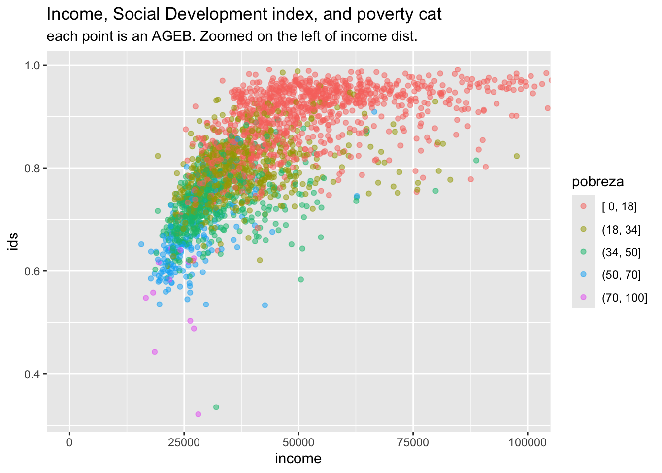 

Some maps as another check

poligonos %>% 
  left_join(ageb_attributes) %>%
  ggplot() +
  geom_sf(aes(fill = income_log_std), color = gray(.2), alpha = .7) +
  annotation_scale(location = "br", style = "ticks") +
  scale_fill_viridis_c() +
  theme_minimal() 

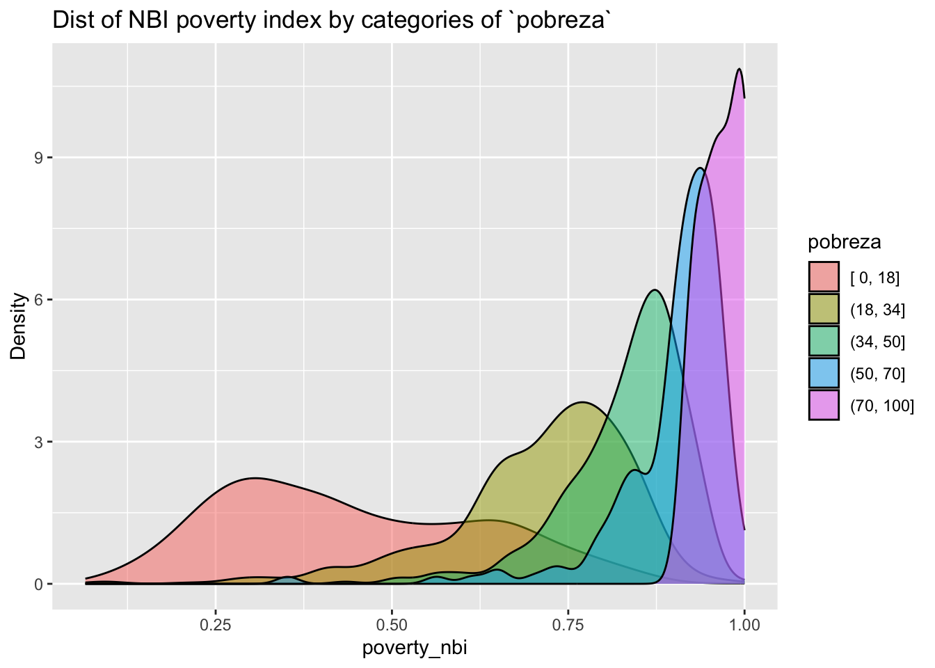
poligonos %>% 
  left_join(ageb_attributes) %>%
  ggplot() +
  geom_sf(aes(fill = ids), color = gray(.2), alpha = .7) +
  annotation_scale(location = "br", style = "ticks") +
  scale_fill_viridis_c() +
  theme_minimal()

poligonos %>% 
  left_join(ageb_attributes) %>%
  ggplot() +
  geom_sf(aes(fill = poverty_nbi), color = gray(.2), alpha = .7) +
  annotation_scale(location = "br", style = "ticks") +
  scale_fill_viridis_c(direction = -1) +
  theme_minimal()

poligonos %>% 
  left_join(ageb_attributes) %>%
  ggplot() +
  geom_sf(aes(fill = pobreza), color = gray(.2), alpha = .7) +
  annotation_scale(location = "br", style = "ticks") +
  scale_fill_viridis_d(direction = -1) +
  theme_minimal()

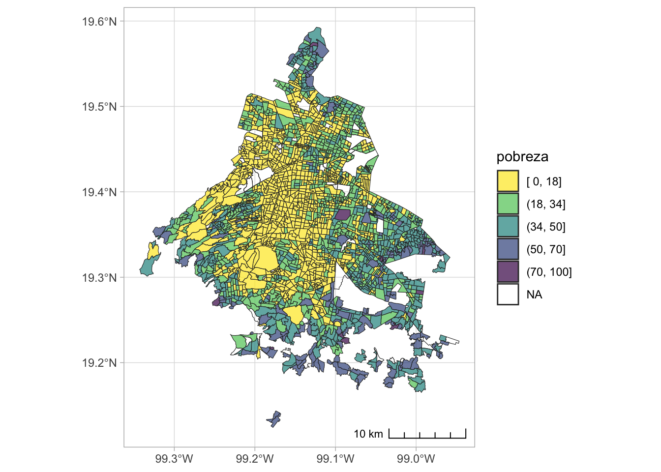
3 Save attributes and borders

ageb_attributes %>% 
  saveRDS(here("..", "output", "ageb_attributes.rds"))

poligonos %>% 
  left_join(ageb_attributes %>% select(ageb, pobtot)) %>% 
  write_sf(here("..", "output", "ageb_poligonos.geojson"),
           delete_dsn = TRUE) #to overwrite