In this script, I process the CONAGUA data for precipitations, measured at daily level for the entire country. I download the relevant station level data in this script.
I then process it, IDW with 20kms cutoff, and save it at the AGEB by day level in processed_conagua_ageb.rds.
(NB: for the most recent data (from second half of 2024), I use a 50kms cutoff to avoid NAs, since the data is more sparse)
I eventually save a file that is at the AGEB by day level, with the daily precipitation.
Download the raw data
This website links all the precipitation data from CONAGUA. https://sih.conagua.gob.mx/climas.html I crawl and download each file. The download would take long because there are almost 8000 files, one for each station over the whole country.
# Extract all the links to CSV filescsv_links <-read_html("https://sih.conagua.gob.mx/climas.html") %>%# Read the webpagehtml_nodes("a") %>%# Select all linkshtml_attr("href") %>%# Extract the href attributestr_subset("\\.csv$") %>%# Keep only the links ending with .csvas_tibble() %>%rename(relative_url = value)
Error in open.connection(x, "rb"): cannot open the connection
The catalog of stations is on the same page. I download it separately.
# download the catalogo# no need to download it again and again# download.file(catalogo_link$url,# here("..", "raw_data", "3_conagua",# "csv_downloaded_by_script_CDMX",# basename(catalogo_link$relative_url)))# import itcatalogo <-read_csv(here("..", "raw_data", "3_conagua","csv_downloaded_by_script_CDMX","0_Catalogo_de_estaciones_climatologicas.csv"),locale =locale(encoding ="ISO-8859-1"))# Clean the column names manuallycolnames(catalogo) <-colnames(catalogo) %>%tolower() %>%# Convert to lowercasestri_trans_general("Latin-ASCII") %>%# Remove accents and special charactersgsub("[^a-z0-9_]", "_", .) %>%# Replace non-alphanumeric characters with "_"gsub("_+", "_", .) %>%# Replace multiple underscores with a single onegsub("_$", "", .) # Remove trailing underscoresrm(catalogo_link)
Select only the stations within 50kms
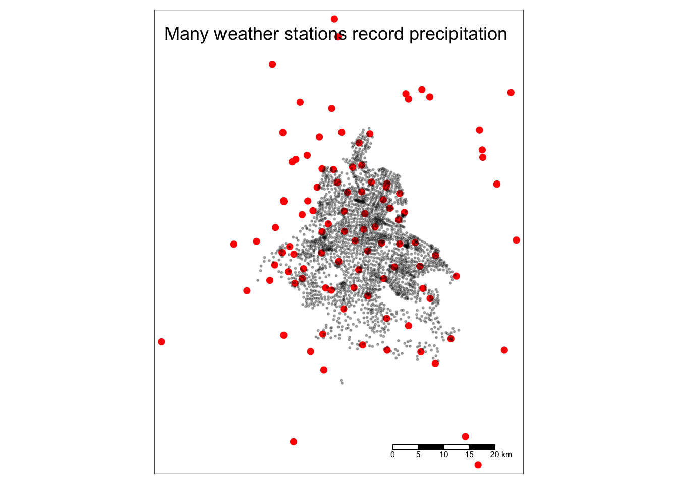
It contains daily measurements for thousands of weather stations across the whole country. I first want to identify the relevant stations for my analysis, i.e. those surrounding CDMX.
I compute the distance of all stations from the geographic center of CDMX. I keep only those located less than 50km away from the center, more than enough. Note, this is not the cutoff for the IDW. Just a first filter.
Filter only the relevant stations, now there are only about 300. Its historical data, so the vast majority of stations will be unused.
And downlaod the data, one by one:
csv_links <- csv_links %>%# remove .csv from filename to get the ID of the stationmutate(clave =str_remove(filename, ".csv"))# keep the links only to the relevant stationscsv_links <- csv_links %>%filter(clave %in% catalogo$clave)# to keep results reproducible, do not add new files# to download fresh files, remove the existing ones first# Check if file already exists, if yes, no need to download it again.# Be polite; ask only once!csv_links %>%filter(!filename %in%list.files(here("..", "raw_data", "3_conagua", "csv_downloaded_by_script_CDMX"))) %>%# Download each filepull(url) %>%walk(~download.file(.x,here("..", "raw_data", "3_conagua","csv_downloaded_by_script_CDMX",basename(.x))),.progress =TRUE)rm(csv_links)
Import the precipitation data
I can now import the data only for those stations.
# list all the filesprec_files <-list.files(here("..", "raw_data", "3_conagua", "csv_downloaded_by_script_CDMX"),full.names = T) %>%as_tibble() %>%rename(full_path = value) %>%mutate(filename =basename(full_path),clave =str_remove(filename, ".csv"))prec_data <-map_dfr(.x = prec_files %>%pull(full_path),.f =~fread(.x,skip =6,# only read date and prec, the rest is incomplete#select = (1:2),na.strings =c("-","")) %>%mutate(clave =str_remove(basename(.x), ".csv")) )# keep only prec and non NA valuesprec_data <- prec_data %>%select(clave,fecha = Fecha,prec =`Precipitación(mm)`) %>%filter(!is.na(prec))rm(prec_files)
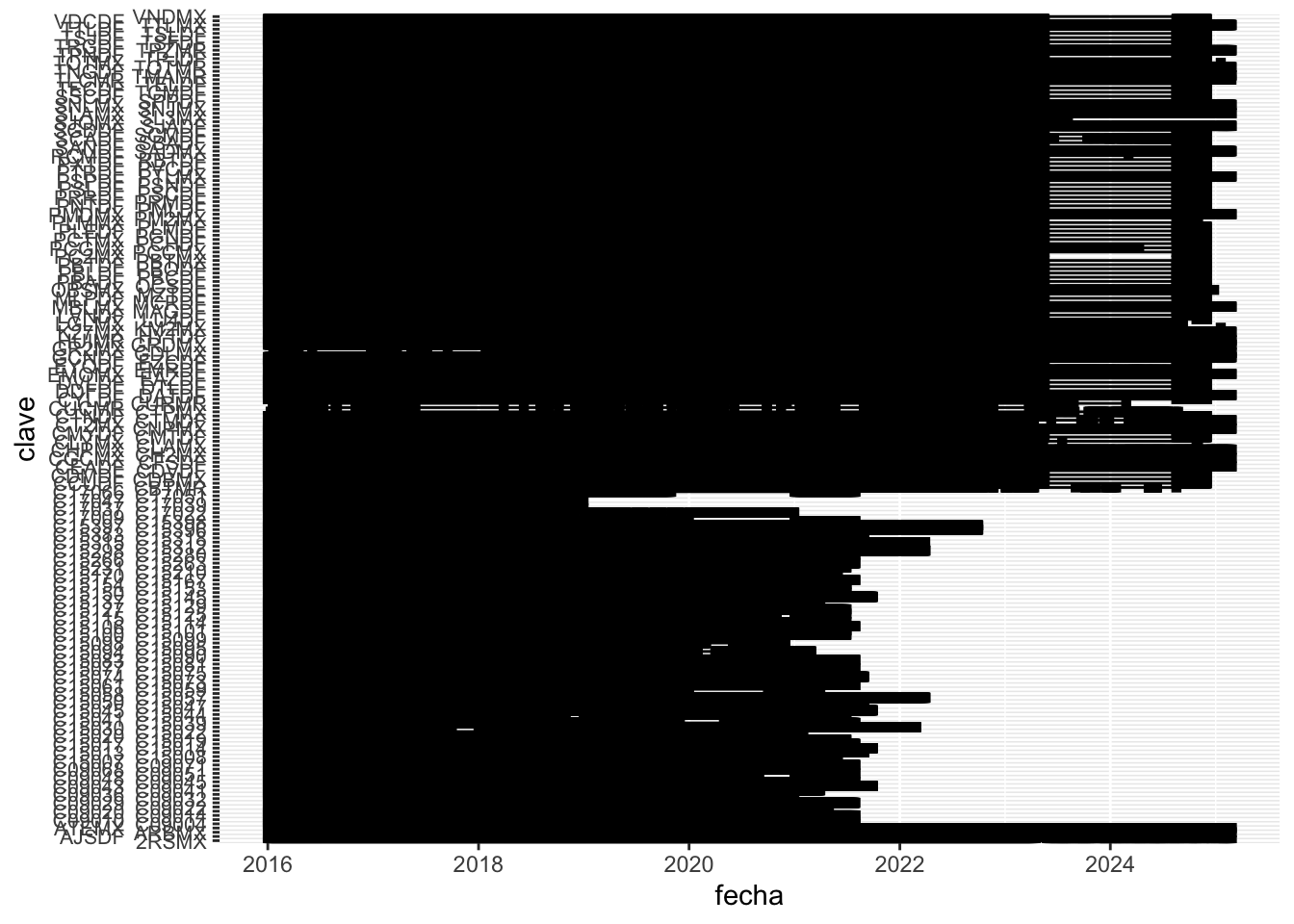
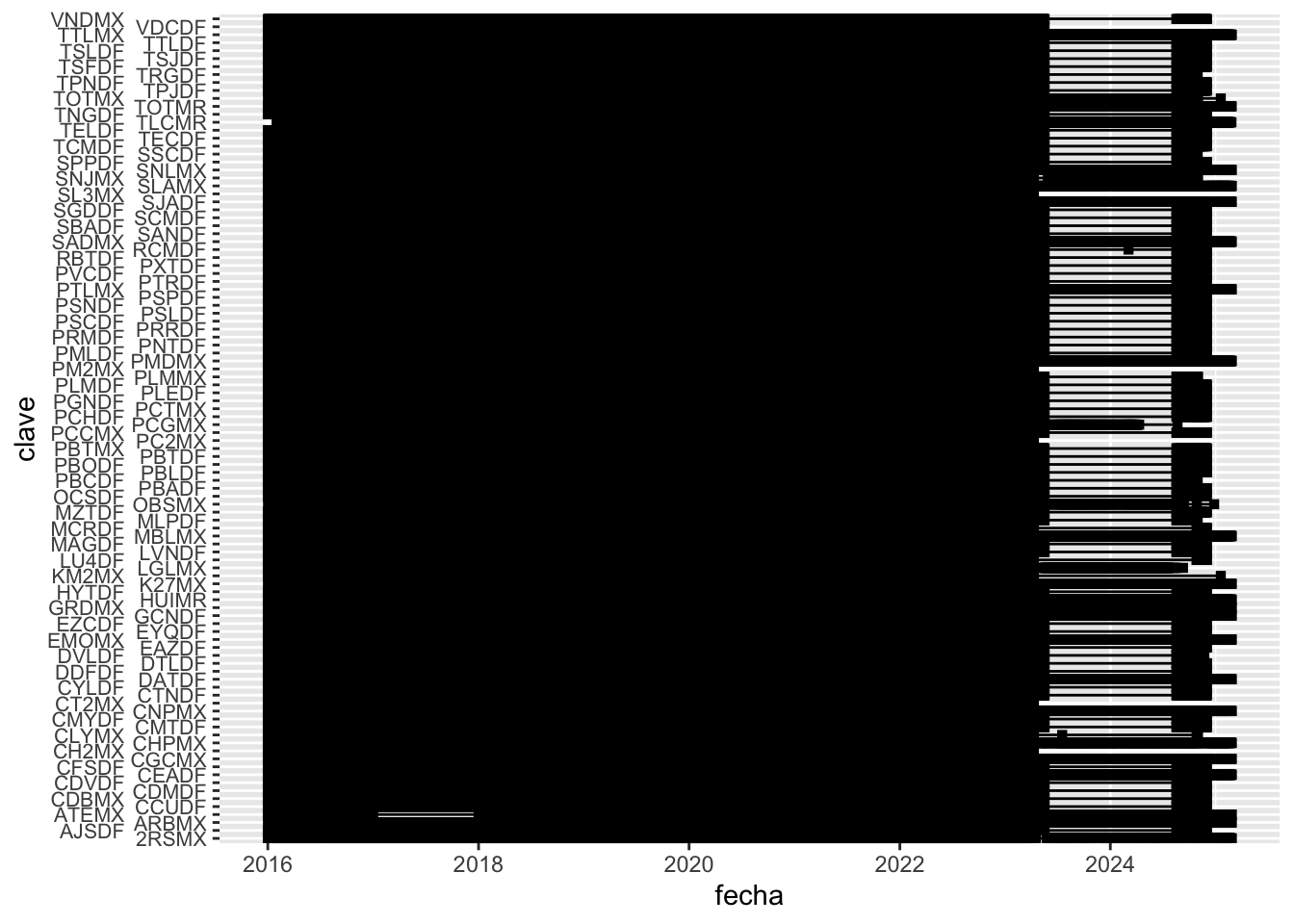
We want to filter the stations that record consistently
station_activity <- prec_data %>%# 9 years, that is 3285 days in totalfilter(year(fecha) %in%2016:2024) %>%# count nr of non NA days per stationgroup_by(clave) %>%summarise(nr_days =n(),share_of_total =100* nr_days/3285) # we keep stations that are active at least 75pc of the timestation_activity <- station_activity %>%filter(share_of_total >=75)catalogo <- catalogo %>%filter(clave %in% station_activity$clave)prec_data <- prec_data %>%filter(clave %in% station_activity$clave)prec_data %>%group_by(fecha) %>%ggplot(aes(x = fecha, y = clave, group = clave)) +geom_line() +geom_point(shape =15) +scale_y_discrete(guide =guide_axis(n.dodge =2)) +theme(axis.text.y =element_text(size =8))
There are many stations recording throughout the whole period, within 50kms of the center. We will only use those within 20km of a CDMX AGEB for the IDW.
I now have to go from stations data to AGEB level.
Compute distances
distances <-crossing( (ageb %>%st_drop_geometry() %>%select(ageb,ageb_lon = lon,ageb_lat = lat)), (catalogo %>%st_drop_geometry() %>%select(clave,sta_lon = longitud,sta_lat = latitud)) ) # compute the distance in meters, using haversine method, and convert to kmdistances <- distances %>%mutate(distance = geosphere::distHaversine(cbind(ageb_lon, ageb_lat),cbind(sta_lon, sta_lat)),distance = distance/1000)distances %>%saveRDS(here("..", "output","temporary_data","weather","distances_precipitation.rds"))
Matching procedure
I have about 3300 days. I have to do it day by day, to not exhaust memory.
# get all the datesfechas <- prec_data %>%pull(fecha) %>%unique()
I assign to each AGEB per day the measures of all stations within 20km. I then compute a distance weighted average for day.
# this long function computes daily averages at the AGEB level# from hourly data at the station level# It also takes care of missing valuesprocess_data_for_one_day <-function(fecha, max_dist) { prec_data_one_day <- prec_data %>%filter(fecha ==!!fecha) one_day <-# take each AGEB and station combination that are within 20km of each other distances %>%filter(distance <= max_dist) %>%select(ageb, clave, distance) %>%# add date to each observationmutate(fecha = prec_data_one_day %>%pull(fecha) %>%unique(), .before =1) %>%# Add the actual data (day x station) to each AGEBleft_join(prec_data_one_day,by =c("clave", "fecha")) %>%filter(!is.na(prec)) %>%# Now, i want to move to the AGEB by date level# I take inverse distance weighted averages, so I compute a weight based on distancemutate(weight =1/distance) %>%group_by(ageb, fecha) %>%# compute idw averagessummarise(prec = stats::weighted.mean(prec, weight, na.rm = T),.groups ="drop")return(one_day)}# just as an example for one day.# I have one observation per AGEB.process_data_for_one_day(fechas[2000], max_dist =20)
# I want to run a lower cutoff ofr IDW for most data,# but a higher cutoff for the most recent days, until# the data gets updated (to avoid NAs) (see station activity above)# We dont want to drop observations just because rain is missing# so i split the date series in two and run the function twicefechas_recent <- fechas[fechas >=as_date("2023-04-01")]fechas_old <-as_date(setdiff(fechas, fechas_recent))# set parallel computingparallel::detectCores()
[1] 10
plan(multisession, workers =6)# set memory limitmem.maxVSize(vsize =40000)
[1] 40000
# run for each daytic()list_of_days_old <-# use map insetad of future_map to run single core with purrrfuture_map(fechas_old, ~process_data_for_one_day(.x, max_dist =20),.progress =TRUE)toc()
prec_daily <-rbind(list_rbind(list_of_days_old),list_rbind(list_of_days_recent) )# fill with NAs for absent combinationsprec_daily <- prec_daily %>%complete(fecha =seq(min(fecha), max(fecha), by ="1 day"), ageb)
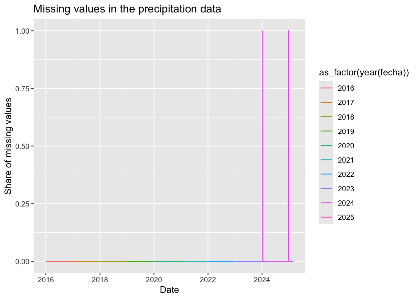
Look at missing values
We only have more sparse data for the recent years (2023, 2024). There are no missing for the earlier years.
With 20km cutoff, we have 54 days in 2023 with some AGEBs missing for precipitation. With 50km, a few days in 2024… Thats why we did it.
missings %>%ggplot(aes(x = fecha, y = share_missing, color =as_factor(year(fecha)))) +geom_line() +labs(title ="Missing values in the precipitation data",x ="Date",y ="Share of missing values")