Heterogeneity: housing

Note

I run the heterogeneity on the housing quality and crowding index (HQCI)

The idea is that:

Housing quality may capture material constraints and exposure/sensitivity better than income alone.
Someone can be low-income but live in high-quality housing and thus be less exposed
In contrast, precarious housing (e.g. tin roofs, crowding) could amplify heat–DV effects even in middle-income areas.

library(tidyverse)
library(here) # path control
library(fixest) # estimations with fixed effects
library(knitr)
library(sf)
library(tictoc)
tic("Total render time")

source("fun_dynamic_bins.R")
source("fixest_etable_options.R")

data <-
  read_rds(here("..", "output", "data_reports.rds")) %>% 
  filter(covid_phase == "Pre-pandemic")

data <- data %>% 
  mutate(prec_quintile = ntile(prec, 5),
         rh_quintile = ntile(rh, 5),
         wsp_quintile = ntile(wsp, 5))

ageb_attributes <- 
  readRDS(here("..", "output", "ageb_attributes.rds"))

poligonos <-  
  read_sf(here("..",
                "output",
                "ageb_poligonos.geojson"),
          quiet = TRUE)

mem.maxVSize(vsize = 40000)

[1] 40000

Describe IDS and compute ntiles

I have a few more variables, discussed in this page, aside from income and poverty. They are from the census.

IDS is índices de desarrollo social. The general one is too wide, it includes health, education, etc.
- ids_ccevj is ids vivienda, this one is more interesting
- I call it Housing Quality and Crowding Index (HQCI)
- It is two dimensional:
  - Calidad de los materiales de la construcción (Walls, roof, flooring)
  - Disponibilidad de espacio en la vivienda (number of rooms, bedrooms, kitchen…) per person in the hh.
GRS is useless, its the census variables again; but through factor analysis etc.

I can relate hqci, poverty and income

ageb_attributes <- ageb_attributes %>% 
  rename(hqci = ids_ccevj)

ageb_attributes %>% 
  # scatter hqci and income
  ggplot(aes(x = income, y = hqci)) +
  geom_point()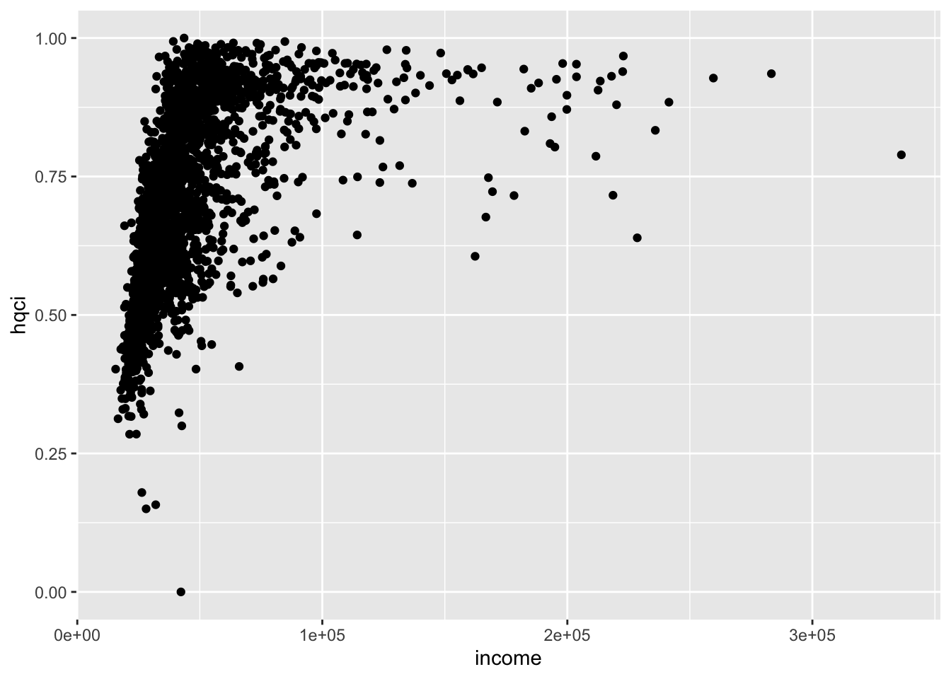

ageb_attributes %>% 
  # scatter hqci and income
  ggplot(aes(x = poverty_nbi, y = hqci)) +
  geom_point()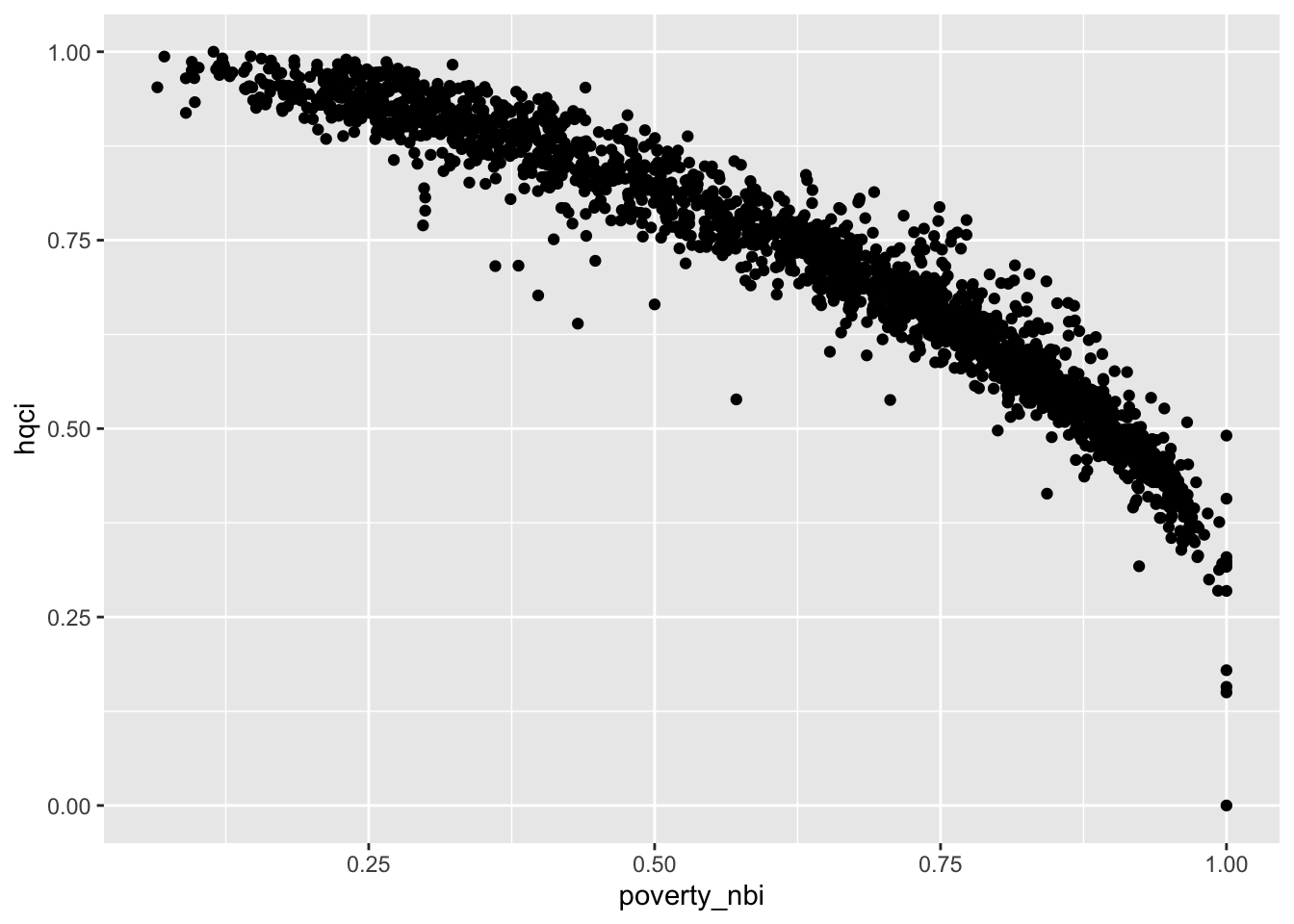

Compute some ntiles of hqci, we weight by AGEB’s population.

ageb_attributes <- ageb_attributes %>% 
  arrange(hqci) %>% 
  mutate(
    # Population-Weighted Deciles
    hqci_decile = ifelse(
      is.na(income) | is.na(pobtot), NA, 
      as_factor(cut(
        cumsum(pobtot[!is.na(hqci)]) / sum(pobtot[!is.na(hqci)], na.rm = TRUE), 
        breaks = seq(0, 1, by = 0.1), 
        labels = 1:10, 
        include.lowest = TRUE
      ))
    )) %>% 
  mutate(
    hqci_quintile = case_when(
      hqci_decile %in% c("1", "2") ~ "1",
      hqci_decile %in% c("3", "4") ~ "2",
      hqci_decile %in% c("5", "6") ~ "3",
      hqci_decile %in% c("7", "8") ~ "4",
      hqci_decile %in% c("9", "10") ~ "5",
      TRUE ~ NA),
    hqci_median = case_when(
      hqci_decile %in% c("1", "2", "3", "4", "5") ~ "Below Median",
      hqci_decile %in% c("6", "7", "8", "9", "10") ~ "Above Median",
      TRUE ~ NA)
  ) %>% 
  mutate(
    hqci_decile = as_factor(hqci_decile),
    hqci_quintile = as_factor(hqci_quintile),
    hqci_median = as_factor(hqci_median)
  )

I plot those new hqci quintiles. Now, the number of AGEB in each is much more balanced (although not equal since we bin by population). We see that it is close but does not correspond to the quintiles of poverty (would be horizontal cuts on the plot).

ageb_attributes %>% 
  ggplot(aes(x = hqci, y = poverty_nbi, color = hqci_quintile)) +
  geom_point() +
  scale_color_brewer(palette = "RdYlBu", direction = -1, na.value = "grey90") +
  theme_minimal()

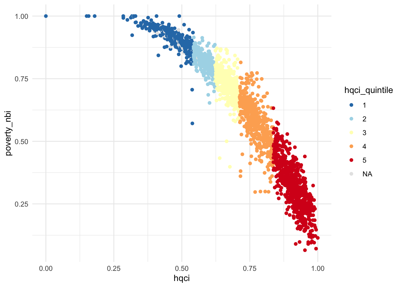
I join these attributes to the main panel

data <- 
  left_join(data, ageb_attributes)

Regressions

Baseline regressions for reference

First the baseline regressions for reference:

baseline_linear <- data %>% 
  fepois(reports_dv ~ tmean |
           prec_quintile + rh_quintile + wsp_quintile +
           ageb + year^month + day_of_week + day_of_year,
         cluster = ~ ageb)

baseline_bins <- data %>% 
  mutate(bins_tmean_one = create_dynamic_bins(tmean, width = 1, 0.01)) %>% 
  fepois(reports_dv ~ i(bins_tmean_one, ref = "[16") |
           prec_quintile + rh_quintile + wsp_quintile +
           ageb + year^month + day_of_week + day_of_year,
         cluster = ~ ageb)

Gradient-style heterogeneity

reg_hqci_cont_linear <- data %>% 
  fepois(reports_dv ~ tmean * hqci |
           prec_quintile + rh_quintile + wsp_quintile +
           ageb + year^month + day_of_week + day_of_year,
         cluster = ~ ageb)

etable(baseline_linear, reg_hqci_cont_linear) %>% 
  kable()

	baseline_linear	reg_hqci_cont_linear
Dependent Var.:	Reports for DV	Reports for DV

Temperature	0.0274*** (0.0033)	0.0512*** (0.0079)
hqci		1.7060 (36,860.9124)
Temperature x hqci		-0.0353*** (0.0107)
Fixed-Effects:	——————	——————–
Prec, hum, wsp quintiles	Yes	Yes
Neighborhood	Yes	Yes
Year-Month	Yes	Yes
Day of Week	Yes	Yes
Day of Year	Yes	Yes
________________________	__________________	____________________
S.E.: Clustered	by: Neighborhood	by: Neighborhood
Observations	3,624,826	3,576,634

Below and above median

reg_above_below_linear <- data %>%
  fepois(reports_dv ~ i(hqci_median, tmean) |
           prec_quintile + rh_quintile + wsp_quintile +
           ageb + year^month + day_of_week + day_of_year,
         cluster = ~ ageb)

etable(baseline_linear, reg_above_below_linear) %>% 
  kable()

	baseline_linear	reg_above_below_..
Dependent Var.:	Reports for DV	Reports for DV

Temperature	0.0274*** (0.0033)
Temperature x hqci_median = BelowMedian		0.0299*** (0.0037)
Temperature x hqci_median = AboveMedian		0.0243*** (0.0037)
Fixed-Effects:	——————	——————
Prec, hum, wsp quintiles	Yes	Yes
Neighborhood	Yes	Yes
Year-Month	Yes	Yes
Day of Week	Yes	Yes
Day of Year	Yes	Yes
_______________________________________	__________________	__________________
S.E.: Clustered	by: Neighborhood	by: Neighborhood
Observations	3,624,826	3,578,253

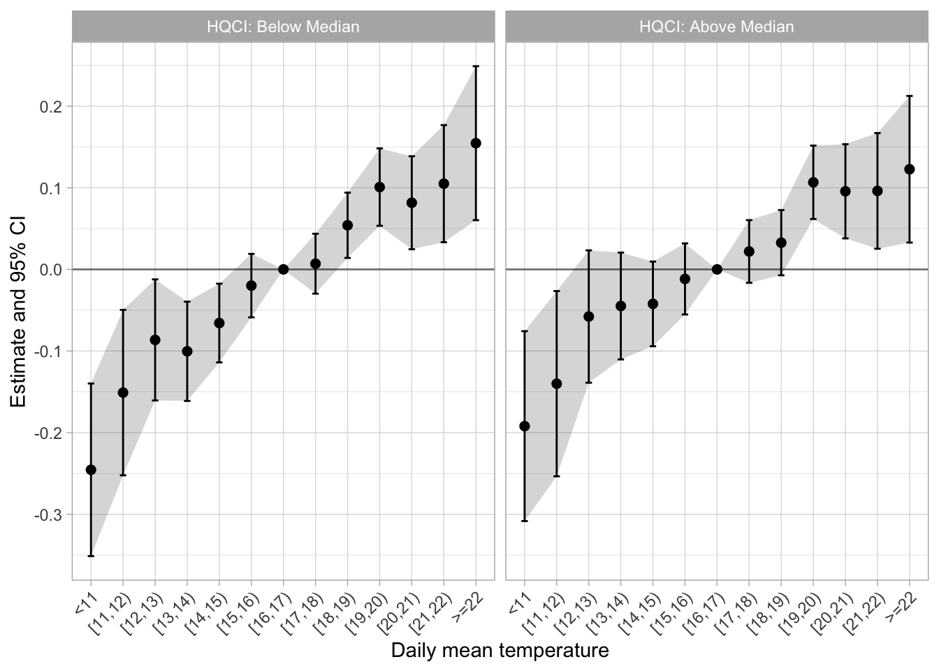
Or semi parametric with bins:

reg_above_below_bins <- data %>%
  mutate(bins_tmean_one = create_dynamic_bins(tmean, width = 1, 0.01)) %>% 
  fepois(reports_dv ~ i(hqci_median, bins_tmean_one, ref2 = "[16") |
           prec_quintile + rh_quintile + wsp_quintile +
           ageb + year^month + day_of_week + day_of_year,
         cluster = ~ ageb)

I can plot these results and save as reg_poverty_median.png

Quintile regressions

I first run the model imposing linearity on tmean and interacting it with poverty quintiles.

reg_quintile_linear <- data %>%
  fepois(reports_dv ~ i(hqci_quintile, tmean) |
           prec_quintile + rh_quintile + wsp_quintile +
           ageb + year^month + day_of_week + day_of_year,
         cluster = ~ ageb)

etable(reg_quintile_linear) %>% 
  kable()

	reg_quintile_lin..
Dependent Var.:	Reports for DV

Temperature x hqci_quintile = 1	0.0311*** (0.0048)
Temperature x hqci_quintile = 2	0.0308*** (0.0044)
Temperature x hqci_quintile = 3	0.0287*** (0.0048)
Temperature x hqci_quintile = 4	0.0288*** (0.0044)
Temperature x hqci_quintile = 5	0.0144** (0.0047)
Fixed-Effects:	——————
Prec, hum, wsp quintiles	Yes
Neighborhood	Yes
Year-Month	Yes
Day of Week	Yes
Day of Year	Yes
_______________________________	__________________
S.E.: Clustered	by: Neighborhood
Observations	3,578,253

Export the table as reg_poverty_quintile.tex

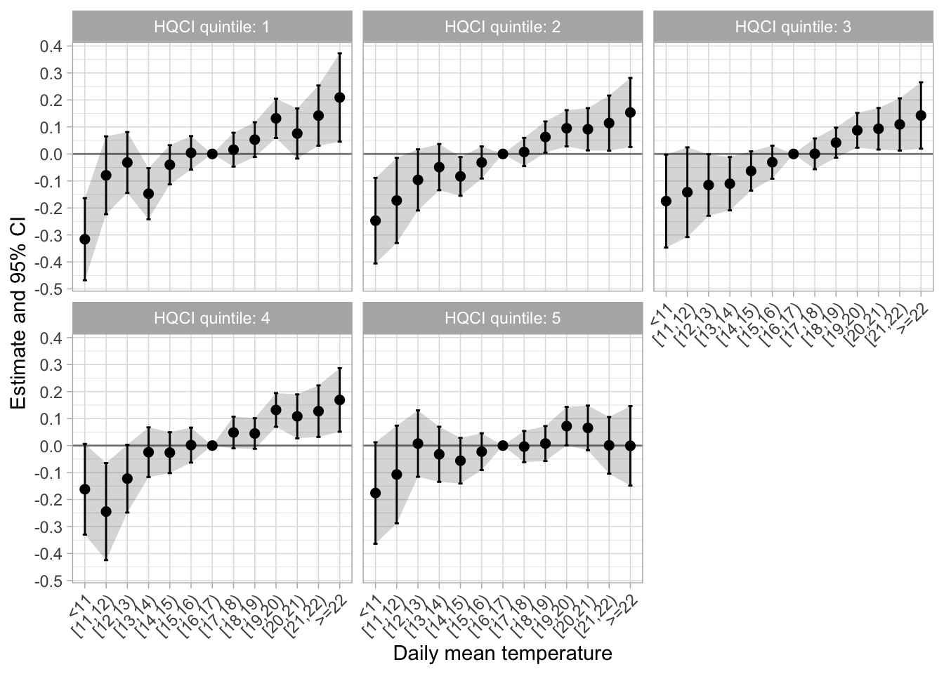
I then allow for possible non-linearities in the relationship between temperature and DV. With the quintiles, its a bit of a crazy estimation…

tic("quintile")
reg_quintile_bins <- data %>%
  mutate(bins_tmean_one = create_dynamic_bins(tmean, width = 1, 0.01)) %>% 
  fepois(reports_dv ~ i(hqci_quintile, bins_tmean_one, ref2 = "[16") |
           prec_quintile + rh_quintile + wsp_quintile +
           ageb + year^month + day_of_week + day_of_year,
         cluster = ~ ageb)
toc()

quintile: 1126.661 sec elapsed

I plot these results.

I save the estimates as reg_HQCI_quintiles_bins_full.png.

Decile

tic("decile")
reg_decile_linear <- data %>%
  fepois(reports_dv ~ i(hqci_decile, tmean) |
           prec_quintile + rh_quintile + wsp_quintile +
           ageb + year^month + day_of_week + day_of_year,
         cluster = ~ ageb)
toc()

decile: 321.38 sec elapsed

etable(reg_decile_linear) %>% 
  kable()

	reg_decile_linear
Dependent Var.:	Reports for DV

Temperature x hqci_decile = 1	0.0292*** (0.0058)
Temperature x hqci_decile = 2	0.0327*** (0.0063)
Temperature x hqci_decile = 3	0.0280*** (0.0056)
Temperature x hqci_decile = 4	0.0333*** (0.0051)
Temperature x hqci_decile = 5	0.0265*** (0.0060)
Temperature x hqci_decile = 6	0.0309*** (0.0058)
Temperature x hqci_decile = 7	0.0303*** (0.0054)
Temperature x hqci_decile = 8	0.0272*** (0.0054)
Temperature x hqci_decile = 9	0.0204*** (0.0059)
Temperature x hqci_decile = 10	0.0075 (0.0060)
Fixed-Effects:	——————
Prec, hum, wsp quintiles	Yes
Neighborhood	Yes
Year-Month	Yes
Day of Week	Yes
Day of Year	Yes
______________________________	__________________
S.E.: Clustered	by: Neighborhood
Observations	3,578,253

iplot(reg_decile_linear)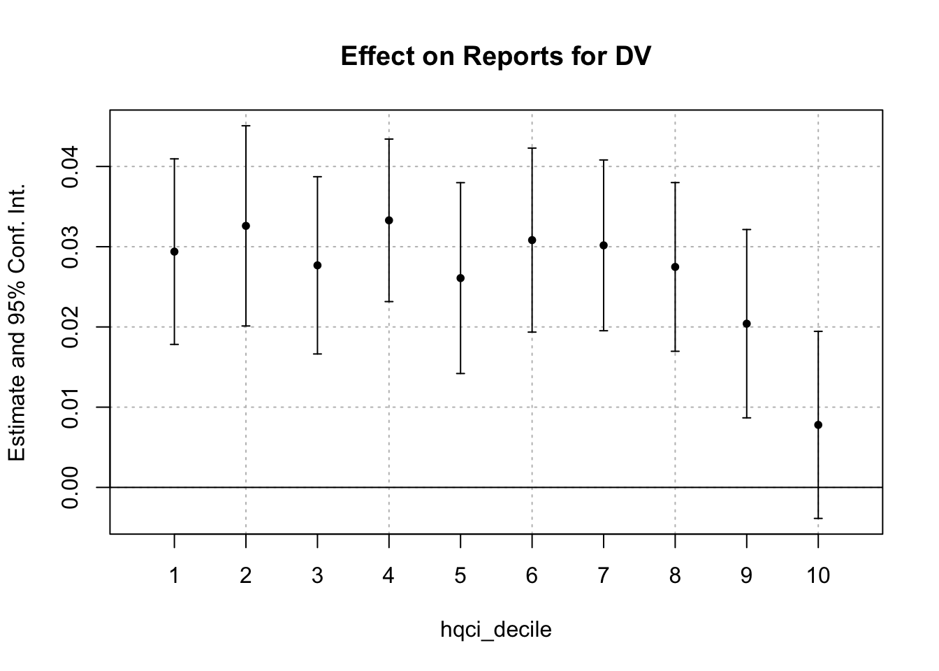

Rendered on: 2025-04-04 19:36:11

Total render time: 2387.842 sec elapsed