servicios_integrales_2016_2018 <-
  fread(here("..", "raw_data",
             "4_locatel",
             "servicios_integrales_2016-2018.csv.zip"),
        colClasses = c(FECHA_ALTA = "character",
                       CP_HECHOS = "character")) %>%
  rename_with(tolower) %>%
  select(-año_alta, -mes_alta, -día_alta, -hora_alta) %>%
  separate(fecha_alta, into = c("fecha_alta", "hora_alta"), sep = "T") %>%
  mutate(hora_alta = str_remove(hora_alta, "Z"))

servicios_integrales_2019_2021 <-
  fread(here("..", "raw_data",
             "4_locatel",
             "servicios_integrales_2019-2021.csv.zip"),
        colClasses = c(FECHA_ALTA = "character",
                       CP_HECHOS = "character")) %>%
  rename_with(tolower) %>%
  select(-año_alta, -mes_alta, -día_alta, -hora_alta)  %>%
  separate(fecha_alta, into = c("fecha_alta", "hora_alta"), sep = "T") %>%
  mutate(hora_alta = str_remove(hora_alta, "Z"))

servicios_integrales_2022_2023 <-
  fread(here("..", "raw_data",
             "4_locatel",
             "servicios_integrales_2022-2023.csv.zip"),
        colClasses = c(fecha_alta = "character",
                       cp_hechos = "character")) %>%
  select(-año_alta, -mes_alta)


locatel <- bind_rows(servicios_integrales_2016_2018,
                     servicios_integrales_2019_2021,
                     servicios_integrales_2022_2023) %>%
  as_tibble()

rm(servicios_integrales_2016_2018,
   servicios_integrales_2019_2021,
servicios_integrales_2022_2023)Helpline data from Línea Mujeres
In this script, I clean the call level data.
- I import the raw data
- I categorise the calls according the the victim/perpetrator of violence and the nature of violence and I select the DV calls.
- I remove the duplicates
- I deal with the locations
The output data is still at the call level. I then plot and describe it.
Import and format the raw call data
Select the period of interest
The date and time are encoded as characters, I encode them as dttm.
locatel <- locatel %>%
  mutate(dttm = ymd_hms(paste(fecha_alta, hora_alta)),
         year = year(dttm),
         month = lubridate::month(dttm, label = F),
         .before = fecha_alta)

locatel %>%
  group_by(year, month) %>%
  summarise(n = n()) %>%
  # plot monthly
  ggplot(aes(month, n)) +
  geom_col() +
  scale_x_continuous(breaks = 1:12) +
  labs(x = NULL,
       y = "Number of calls") +
  facet_wrap(~year)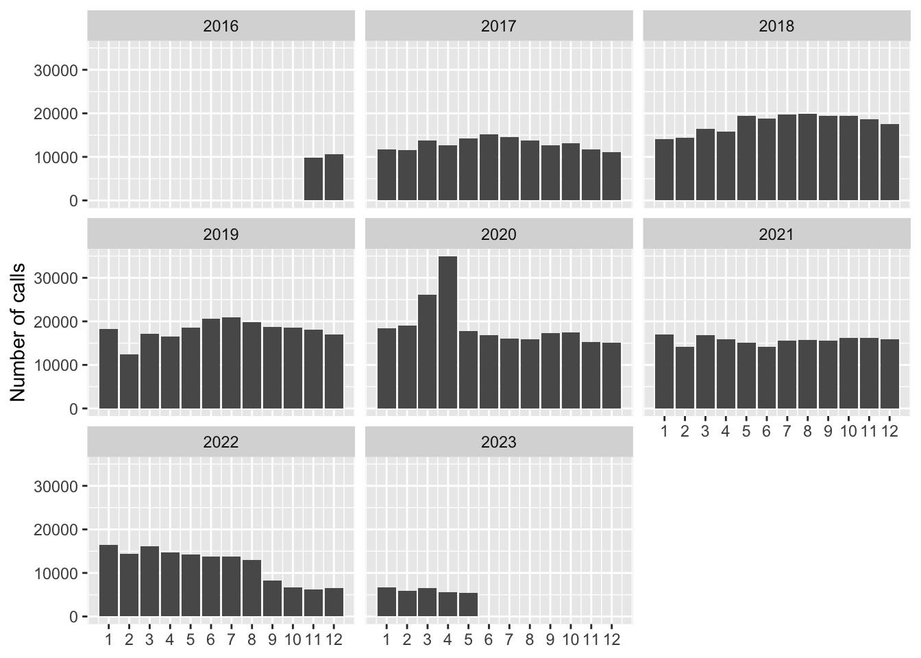
I select the calls from the beginning of the dataset (November 2016) to the end. The drop from September 2022 makes me doubt the fact that it is complete, like they say. So i exclude these months.
locatel <- locatel %>%
  filter(dttm >= ymd("2016-11-01") & dttm < ymd("2022-09-01"))
Also, to explain the drop in feb 2019:
Durante el periodo del 8 a 14 de febrero de 2019 se presentaron problemas técnicos con el sistema SIRILO que impidió la captura de la información; sin embargo, las asesorías se siguieron proporcionando de manera normal durante este periodo, sin afectar la calidad de atención proporcionada a las usuarias.
#remove those days
locatel <- locatel %>%
  filter(!(year == 2019 & month == 2 & day(dttm) %in% 8:14))
Geolocalise the calls
In the call data, the only geographic information I have is the names of the district and neighborhoods. I need to match those names to the ones I got from the CONAPO data.
conapo <-
  read_sf(here("..", "output",
               "colonias.gpkg"))
Uniquely identify each locations in the call data
I want to have a list of all possible combinations of names that appear in the call data. First, I remove the accents from all the location names in the call data.
locatel <- locatel %>%
  mutate(across(c("estado_usuaria", "municipio_usuaria", "colonia_usuaria",
                  "estado_hechos", "municipio_hechos", "colonia_hechos"),
                ~ stringi::stri_trans_general( .x, "Latin-ASCII")))
First, I get all possible combinations of locations for both users and incidents and create a unique ID for each possible locations.
location_usuaria <- locatel %>%
  count(estado = estado_usuaria,
        municipio = municipio_usuaria,
        colonia = colonia_usuaria,
        name = "n_usuaria")

location_hechos <- locatel %>%
  count(estado = estado_hechos,
        municipio = municipio_hechos,
        colonia = colonia_hechos,
        name = "n_hechos")

call_locations <-
  full_join(location_usuaria, location_hechos) %>%
  mutate(id_col_call = row_number() + 70000)


rm(location_usuaria, location_hechos)
So now, I have a list of each locations with a unique ID, id_col_call.
I assign this unique code back to the call data.
locatel <- call_locations %>%
  select(-"n_usuaria",-"n_hechos") %>%
  rename(id_col_call_usuaria = id_col_call,
         estado_usuaria = estado,
         municipio_usuaria = municipio,
         colonia_usuaria = colonia) %>%
  right_join(locatel)

locatel <- call_locations %>%
  select(-"n_usuaria",-"n_hechos") %>%
  rename(id_col_call_hechos = id_col_call,
         estado_hechos = estado,
         municipio_hechos = municipio,
         colonia_hechos = colonia) %>%
  right_join(locatel)
At this point, I still have calls that could originate from outside of CDMX. I keep only the CDMX ones.
locatel <- locatel %>%
  filter(estado_hechos == "CIUDAD DE MEXICO" |
           estado_usuaria == "CIUDAD DE MEXICO")
Match colonias in the call data and colonias of CONAPO
At this point, I have my reference colonias from the CONAPO on the one hand and the list of all possible locations for the call data. I want to match those two sources based on the names of colonias.
I keep only call locations within CDMX.
call_locations <- call_locations %>%
  filter(estado == "CIUDAD DE MEXICO") %>%
  select(-"estado", -"n_hechos")
For that purpose, I want to create a join table for a one-to-many join. Each entry from the CONAPO dataset (identified by the col_id) can be matched to either 0, 1 or more colonias from the call data.
I bind all the locations from both source into the same dataframe. Each row corresponds to a colonia, either in the CONAPO data, or in the call data.
join_table <-
  conapo %>%
  st_drop_geometry() %>%
  select(col_id, municipio = nom_mun, colonia, pobtot) %>%
  mutate(pobtot = round(pobtot)) %>%
  mutate(across(where(is.character),
                ~ toupper(stringi::stri_trans_general( .x, "Latin-ASCII")))) %>%
  bind_rows(., call_locations, .id = "source") %>%
  mutate(source = ifelse(source == 1, "conapo", "call")) %>%
  as_tibble() %>%
  arrange(municipio, colonia) %>%
  relocate(source, col_id,
           colonia, municipio, pobtot, n_usuaria,
           id_col_call)
I create a match key, based on a match with names.
join_table <- join_table %>%
  group_by(municipio, colonia) %>%
  mutate(match_key = ifelse(n() == 2, mean(col_id, na.rm = T), col_id),
         .after = col_id) %>%
  arrange(municipio, colonia)
In this join table, each row corresponds to a location, either in the CONAPO data, or in the call data. For example, the first two rows correspond to the same colonia. So, they have the same match key. However, rows 5 and 6 also corresponds to the same colonia, but since their names differ because the abbreviation is different, they do not have a common match key yet. Since a fuzzy maching technique would take too long, I decide to match them manually.
I export the join table to excel so that I can edit it manually.
join_table %>%
#  group_by(municipio) %>%
#  group_split() %>%
  write_xlsx(path = here("..",
                         "raw_data",
                         "4_locatel",
                         "_join_table",
                         "join_table.xlsx"))
I assigned the match keys manually. I checked using the map, and matched names using abbreviations etc…
Import the edited join table.
join_table <-
  read_excel(here("..",
                  "raw_data",
                  "4_locatel",
                  "_join_table",
                  "join_table_edited_manually.xlsx"))
There are colonias from the call data that are not matched to any colonia in the CONAPO reference data. This is because the name of the colonia in the call data is wrong, i.e. it does not refer to a colonia, but for example to ‘center’ or a public administration etc… Still, 94pc of calls are matched to a colonia in the CONAPO data.
join_table %>%
  filter(source == "call") %>%
  group_by(is.na(match_key)) %>%
  summarise(calls = sum(n_usuaria)) %>%
mutate(prop = 100 * calls / sum(calls)) %>% kable()| is.na(match_key) | calls | prop |
|---|---|---|
| FALSE | 842874 | 93.850274 |
| TRUE | 55231 | 6.149726 |
Overall, 25pc of the colonias in the call data are not matched to any colonia in the CONAPO data. We discard these calls. About 70pc of the call locations are matched 1-to-1 to a colonia in the CONAPO data.
join_table %>%
  count(match_key, source) %>%
  pivot_wider(names_from = "source",
              values_from = n) %>%
  count(call, conapo, sort = T) %>%
  mutate(prop_pc = 100 * n / sum(n),
         cumprop = cumsum(prop_pc)) %>%
kable()| call | conapo | n | prop_pc | cumprop |
|---|---|---|---|---|
| 1 | 1 | 1334 | 68.4453566 | 68.44536 |
| NA | 1 | 485 | 24.8845562 | 93.32991 |
| 2 | 1 | 106 | 5.4386865 | 98.76860 |
| 3 | 1 | 14 | 0.7183171 | 99.48692 |
| 5 | 1 | 2 | 0.1026167 | 99.58953 |
| 4 | 1 | 1 | 0.0513084 | 99.64084 |
| 6 | 1 | 1 | 0.0513084 | 99.69215 |
| 7 | 1 | 1 | 0.0513084 | 99.74346 |
| 8 | 1 | 1 | 0.0513084 | 99.79477 |
| 9 | 1 | 1 | 0.0513084 | 99.84607 |
| 11 | 1 | 1 | 0.0513084 | 99.89738 |
| 15 | 1 | 1 | 0.0513084 | 99.94869 |
| 387 | NA | 1 | 0.0513084 | 100.00000 |
Recode the location identifier in the call data
Now, I want to replace the location data with the new match_key, so that I can locate the calls with reference to the CONAPO data.
First, remove the old location information, and keep only the identifier.
locatel <- locatel %>%
  select(-"estado_hechos", -"municipio_hechos", -"colonia_hechos",
         -"estado_usuaria", -"municipio_usuaria", -"colonia_usuaria")
Then match with the new match_key.
#for usuaria
locatel <-
  join_table %>%
  filter(source == "call") %>%
  select(id_col_call_usuaria = id_col_call,
         col_id_usuaria = match_key) %>%
  right_join(locatel) %>%
  select(-id_col_call_usuaria)

#and for hechos
locatel <-
  join_table %>%
  filter(source == "call") %>%
  select(id_col_call_hechos = id_col_call,
         col_id_hechos = match_key) %>%
  right_join(locatel) %>%
  select(-id_col_call_hechos)
Hechos and usuaria
The location of the user, i.e. the caller, is always reported. Importantly, if e.g. the caller is not the victim, the location of the event can differ from the location of the caller. In that case, it is possible to record a second location, the one where the event took place.
As explained in Locatel’s documentation, in a lot of cases, the event’s location corresponds to the caller’s location, and is thus only recorded once. However, when the event’s location is missing, there is no way to tell if it is because both locations are the same or if it is different and not reported.
This table shows that 80% of events’ location is missing.
locatel %>%
  count(missing_event = is.na(col_id_hechos),
        missing_user = is.na(col_id_usuaria)) %>%
mutate(freq = 100 * n / sum(n)) %>% kable()| missing_event | missing_user | n | freq |
|---|---|---|---|
| FALSE | FALSE | 118077 | 13.4249348 |
| FALSE | TRUE | 6475 | 0.7361845 |
| TRUE | FALSE | 581114 | 66.0705941 |
| TRUE | TRUE | 173869 | 19.7682867 |
If we look at the calls for which both locations are recorded, in 82pc of the cases, the colonia is the same for the caller than for the victim. In 90, both locations are within the same municipio. This could be the victim reporting herself, or a neighbor calling, a teacher, a family member…
locatel %>% filter(!is.na(col_id_hechos)) %>%
  count(same_location = col_id_hechos == col_id_usuaria) %>%
mutate(freq = 100 * n / sum(n)) %>% kable()| same_location | n | freq |
|---|---|---|
| FALSE | 17732 | 14.236624 |
| TRUE | 100345 | 80.564744 |
| NA | 6475 | 5.198632 |
Select general DV calls and create categorise using call topics (tematicas)
Locatel offers many services and thus reasons to call. I want to select the calls that concern domestic violence. The reasons for the call are broken down in 7 categories. There are 3250 possible combinations of the 7 categories, according to the data dictionary. However, there are a bit more in the actual data.
Aviso: A partir de noviembre de 2020 la base de datos de Línea Mujeres se completó para mostrar todos los servicios ofrecidos para la población en general. This is retroactive.
So I need to select only the relevant calls.
I find all possible combinations of categories and count calls in each:
tematicas <- locatel %>%
  count(servicio,
        tematica_1,
        tematica_2,
        tematica_3,
        tematica_4,
        tematica_5,
        tematica_6,
        tematica_7) %>%
  mutate(prop = 100 * n / sum(n))
I also to mark all the combination of categories for which any of the tematica contains the word violencia.
tematicas <- tematicas %>%
  mutate(word_violencia = if_any(starts_with("tematica"),
                                ~ grepl("VIOLENCIA", .x, fixed = TRUE) == TRUE),
         .before = servicio)
There are 868 categories that contain the word violencia. NB: I don’t classify according to this criteria, this is just for information.
Within those, I want to identify those that refer to domestic violence. Since there are so many categories, and they are all messed up, its hard to figure out a proper system. I have tried many things from here. Eventually, I figured that the simplest is to export the list and create the categories manually, and then import it back in.
writexl::write_xlsx(tematicas,
                    here("..", "raw_data",
                         "4_locatel",
                         "my_tematicas.xlsx"))
tematicas <- read_xlsx(here("..", "raw_data",
"4_locatel",
"my_tematicas_edited.xlsx"))I join this new categorization to the call level data. And I exclude all the calls that are not domestic violence.
locatel <- locatel %>%
  left_join(tematicas) %>%
  filter(DV == "domestic violence") %>%
  select(-"n", -"prop", -"prop selected", -"word_violencia", -"marked")

rm(tematicas)
I divide domestic violence into broad categories according to who are the perpetrators and victims of violent acts: 1. Intimate partner violence 2. Violence committed by family members (other than partner) 3. Violence against children 4. Violence against adult
By looking more closely at the nature of acts of violence, these three categories can be further divided into three types of violence: 1. Physical violence 2. Sexual violence 3. Psychological violence
I want to visualise the categories using a Sankey diagram:
locatel %>% count(DV, TYPE, NATURE) %>% kable()| DV | TYPE | NATURE | n |
|---|---|---|---|
| domestic violence | intimate partner violence | physical | 4038 |
| domestic violence | intimate partner violence | psychological | 12967 |
| domestic violence | intimate partner violence | sexual | 270 |
| domestic violence | intimate partner violence | unknown | 587 |
| domestic violence | unknown | unknown | 17669 |
| domestic violence | violence against adult | unknown | 24702 |
| domestic violence | violence against children | physical | 2208 |
| domestic violence | violence against children | psychological | 977 |
| domestic violence | violence against children | sexual | 524 |
| domestic violence | violence against children | unknown | 4047 |
| domestic violence | violence committed by family members | physical | 1378 |
| domestic violence | violence committed by family members | psychological | 3105 |
| domestic violence | violence committed by family members | sexual | 340 |
locatel %>%
  ggsankey::make_long(DV, TYPE,  NATURE) %>%
  ggplot(., aes(x = x, next_x = next_x, node = node,
                next_node = next_node,
                fill = factor(node), label = node)) +
  geom_sankey(flow.alpha = .6,
              node.color = "gray30") +
  geom_sankey_label(size = 3, color = "white", fill = "gray40") +
  scale_fill_viridis_d() +
  theme_sankey(base_size = 12) +
  labs(x = NULL) +
  theme(legend.position = "none")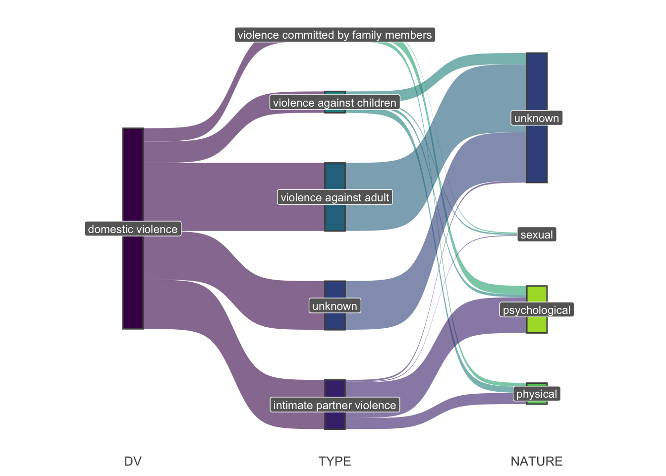
Remove duplicates
There are 72812 DV calls in the data for CDMX. Supposedly, folio is the Identificador único de la llamada. However, it is not unique. It is sometimes used for multiple observations, which however differ on the rest of the characteristics. My guess is that the system assigns ids based on time, and if two calls get recorded at the same moment, they might duplicate. I thus remove this variable and create a new unique id_number.
nrow(locatel)[1] 72812nrow(locatel %>% distinct(folio))[1] 70586locatel <- locatel %>%
select(-folio) %>%
rownames_to_column(var = "unique_id") %>%
mutate(unique_id = as.numeric(unique_id))Multiple entries
Still, there are some real duplicate entries. I consider observations as duplicate if all these variables are exactly the same in two entries.
dupes <- locatel %>%
  get_dupes(fecha_alta, sexo, edad, estado_civil, ocupacion, escolaridad,
            col_id_usuaria,
            col_id_hechos,
            origen, servicio, tematica_1, tematica_2, tematica_3,
            tematica_4, tematica_5, tematica_6, tematica_7)
There are 5078 duplicates. They are multiple entries in the system, recorded a few seconds apart. I don’t want to remove all the 5078 duplicates, but keep one observation for each group of duplicates.
# This keep all variables in "dupes" but if
# a combination of fecha_alta:dupe_count is not distinct,
# this keeps the first row of values.

dupes_to_keep <- dupes %>%
  distinct(across(fecha_alta:dupe_count), .keep_all = T) %>%
  select(-dupe_count)
I now remove those duplicates from the locatel data
dupes_to_dump <- anti_join(dupes, dupes_to_keep, by = "unique_id")

locatel <- locatel %>%
  filter(! unique_id %in% dupes_to_dump$unique_id)

rm(dupes, dupes_to_dump, dupes_to_keep)
I have 70238 unique calls.
Same caller on the same day
One last issue to take care of is that I might have multiple calls for the same event. I check when there are multiple calls for the same day and same user. Usually, the caller is redirected to another service, and the call is entered in the system another time.
dupes <- locatel %>%
  get_dupes(fecha_alta, # same day
            sexo, edad, estado_civil, ocupacion, escolaridad, # same user characteristics
            col_id_usuaria, # same user location
            col_id_hechos # same event location
            )

# I create a group per each event. A group contains two or three calls
dupes <- dupes %>%
  group_by(fecha_alta, # same day
           sexo, edad, estado_civil, ocupacion, escolaridad, # same user characteristics
           col_id_usuaria, # same user location
           col_id_hechos # same event location
  )
Out of the multiple calls (i.e. group), I want to keep the call that provides me with the best level of detail as to what type of crime it is. I sort by group, NAs go last, and I keep the first observation of each group.
dupes_to_keep <- dupes %>%
  mutate(across(c("TYPE", "NATURE"), ~ na_if(., "unknown"))) %>%
  arrange(TYPE, NATURE, .by_group = TRUE) %>%
  filter(row_number(fecha_alta) == 1)
Remove the multiple calls for the same events from the call data
dupes_to_dump <- anti_join(dupes, dupes_to_keep, by = "unique_id")

locatel <- locatel %>%
  filter(!unique_id %in% dupes_to_dump$unique_id)

rm(dupes, dupes_to_dump, dupes_to_keep)
Save the call-level data
locatel %>% saveRDS(here("..", "output",
                         "temporary_data",
                         "dv",
                         "locatel.rds"))
Plot the call-level data
locatel <- readRDS(here("..", "output",
                        "temporary_data",
                        "dv",
                        "locatel.rds"))
Plot hourly distribution of calls
locatel %>%
  count(hour = hour(dttm)) %>%
#  mutate(n = 100*`Number of calls`/sum(`Number of calls`)) %>%
  ggplot(aes(hour, n)) +
  geom_col() +
  scale_x_continuous(breaks=0:23) +
  labs(x = element_blank(),
       y = element_blank())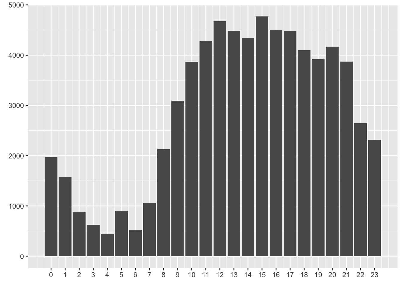
locatel %>%
  count(`Week day` = lubridate::wday(dttm, label = T, week_start = 1)) %>%
#  mutate(n = 100*n/sum(n)) %>%
  ggplot(aes(`Week day`, n)) +
  geom_col() +
  labs(x = element_blank(),
       y = element_blank())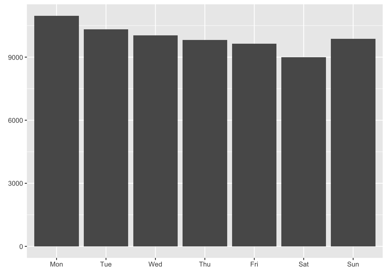
locatel %>%
  mutate(`Age group` = cut(edad,
                           breaks = c(-100, 20, 30, 40, 50, 60, 70, 200),
                           right = F)) %>%
  mutate(`Age group` = fct_recode(`Age group`,
                                  "<20"    = "[-100,20)",
                                  ">=70"      = "[70,200)")) %>%
  count(`Age group`) %>%
#  mutate(n = 100*n/sum(n)) %>%
  ggplot(aes(`Age group`, n)) +
  geom_col() +
  ylab("")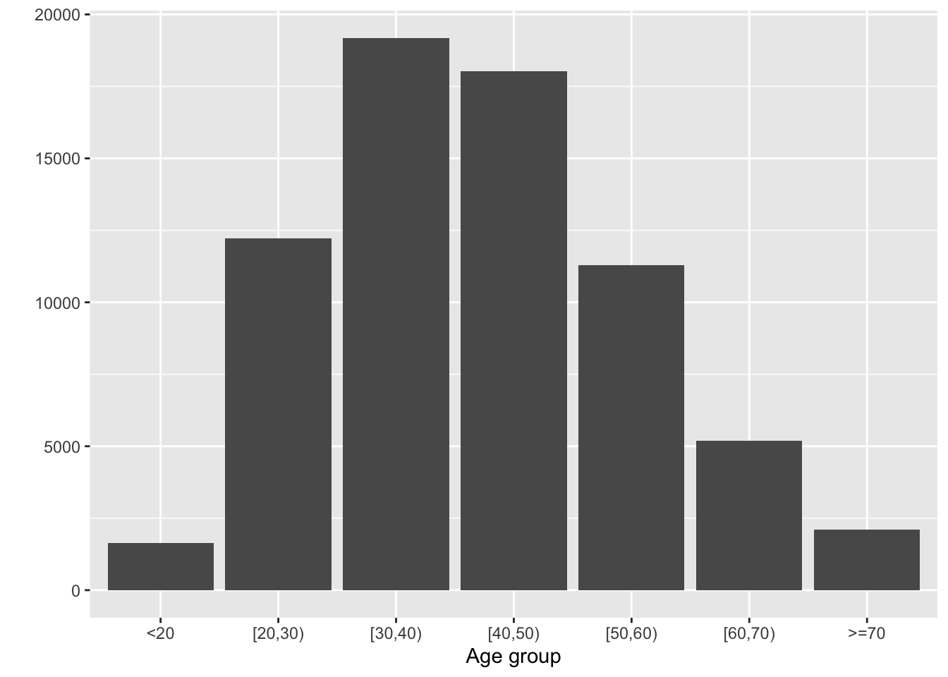
Calls are distributed quite equally over the days of the week and that calls are placed mostly during work hours, and in the evening.
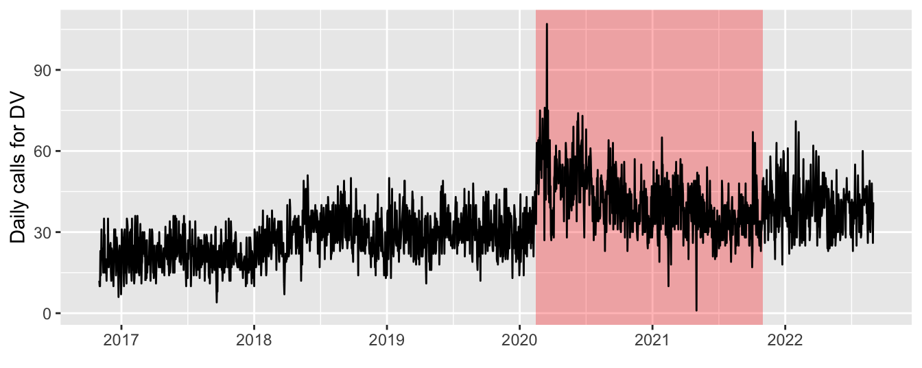
locatel %>%
  mutate(fecha_alta = decimal_date(as_date(fecha_alta))) %>%
  count(fecha_alta) %>%
  ggplot() +
    geom_rect(data = data.frame(xmin = decimal_date(as.Date(c("2020-02-15"))),
                              xmax = decimal_date(as.Date(c("2021-11-01"))),
                              ymin = -Inf,
                              ymax = Inf),
            aes(xmin = xmin, xmax = xmax, ymin = ymin, ymax = ymax),
            fill = "red", alpha = 0.3) +
  geom_line(aes(fecha_alta, n), colour = "black", stat = 'identity') +
  scale_x_continuous(breaks = 2016:2023) +
  labs(x = element_blank(),
       y = "Daily calls for DV")