poligonos <-
  read_sf(here("..", "output", "ageb_poligonos.geojson"),
          quiet = TRUE)

colonias <-
  read_sf(here("..", "output", "colonias.gpkg"),
          quiet = TRUE)

calls <-
  read_rds(here("..", "output", "temporary_data", "dv", "locatel.rds")) %>%
  mutate(date = as_date(fecha_alta),
         hour = as.numeric(str_sub(hora_alta, 1, 2)),
         .keep = "unused")

reports <-
  read_rds(here("..", "output", "temporary_data", "dv", "PGJ_carpetas.rds")) %>%
  st_drop_geometry() %>%
  mutate(hour = lubridate::hour(dttm))

weather <-
  read_rds(here("..", "output", "temporary_data", "weather", "weather_cdmx.rds")) %>%
mutate(date = ymd(date)) Count, bin, and merge data sources
Note
In this script, I import the reports, calls, weather, and pollution data.
I count the reports/calls per day, per AGEB/neighborhood. I also split e.g. per type of crime, per time of day etc.
I then create bins with the weather data.
I merge all the data sources into two final datasets that I use for regressions:
data_reports.rdswhich is at the AGEB per day leveldata_calls.rdswhich is at the neighborhood per day level
Import the pre-processed data
Time dimension
Create a complete time dataset
I start by creating a dataset for the time dimension, at the day level.
# I create an ageb x day level data, that I populate along the way
# 2,922 days and 1,948 colonias
time <- expand_grid(
  date = seq(ymd("2016-01-01"), ymd("2024-12-31"), by = "days")
  ) %>%
  as_tibble()
I then add variables for the fixed effects, e.g. day of week, month, weekend dummy…
# Create some useful time variables
time <- time %>%
  mutate(year = year(date),
         month = lubridate::month(date, label = T),
         day = lubridate::day(date),
         day_of_week = lubridate::wday(date, label = T),
         day_of_year = paste(lubridate::mday(date),
                             lubridate::month(date, label = T), sep = "-"),
         weekend_dummy = ifelse(day_of_week %in% c("Sat", "Sun"),
                          "Weekend",
                          "Weekdays"),
         calendar_day = paste(month, day))
Pandemic timeline
I set the pandemic period and create a variable. Here is a timeline of data coverage and covid phases.
#My own indicators of covid_phases, based on the COVID appendix
time <- time %>%
  mutate(covid_phase = case_when(date >= ymd("2021-11-01") ~ "Post-pandemic",
                                 date >= ymd("2020-02-15") ~ "Pandemic",
                                 .default = "Pre-pandemic"))

time %>% select(date, covid_phase) %>%
  group_by(covid_phase) %>%
  summarise(start_date = min(date), end_date = max(date)) %>%
mutate(n_days = end_date- start_date) %>% arrange(start_date) %>% gt()| covid_phase | start_date | end_date | n_days |
|---|---|---|---|
| Pre-pandemic | 2016-01-01 | 2020-02-14 | 1505 |
| Pandemic | 2020-02-15 | 2021-10-31 | 624 |
| Post-pandemic | 2021-11-01 | 2024-12-31 | 1156 |
Data coverage timeline
time %>%
  select(date, covid_phase) %>%
  group_by(covid_phase) %>%
  summarise(start = min(date), end = max(date)) %>%
  rename(phase = covid_phase) %>%
  mutate(ymin = 0, ymax = 100, ymed = 50)  %>%
  add_row(phase = "Call data" ,
          start = as_date(min(calls$date)),
          end = as_date(max(calls$date)),
          ymin = 120, ymax = 220,  ymed = 170) %>%
  add_row(phase = "Crime data" ,
          start = as_date(min(reports$date)),
          end = as_date(max(reports$date)),
          ymin = 240, ymax = 340,  ymed = 290) %>%
  add_row(phase = "Weather data" ,
          start = as_date(min(weather$date)),
          end = as_date(max(weather$date)),
          ymin = 360, ymax = 460,  ymed = 410) %>%
  mutate(median = start + (end - start)/2) %>%
ggplot(aes(xmin = start, xmax = end, ymin = ymin, ymax = ymax, fill = phase)) +
  geom_rect(colour = "white") +
  scale_fill_brewer(palette = "Set3") +
  geom_text(aes(x = median, y = ymed, size = .3, label = phase)) +
  xlab(NULL) +  ylab(NULL) +
  scale_x_date(breaks = "years", date_labels = "%d %b %y ") +
  theme(axis.text.y = element_blank(),
        axis.ticks.y = element_blank()) +
  theme(legend.position = "none") +
  guides(x = guide_axis(angle = 45))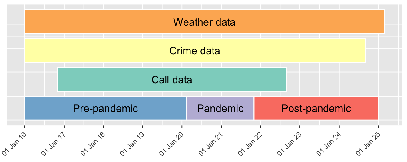
Holidays and school holidays
Import the holiday days and create a dummy in the dataset. I do not have school holidays (yet) because it’s a bit cumbersome.
public_holidays <-
  list.files(here("..", "raw_data", "8_holidays"),
             pattern = "csv", full.names = T) %>%
  map_dfr(read_csv)

public_holidays %>% filter(year(Date) == 2016) %>%
kable()| Date | LocalName | Name | CountryCode | Fixed | Global | LaunchYear | Type | Counties |
|---|---|---|---|---|---|---|---|---|
| 2016-01-01 | Año Nuevo | New Year’s Day | MX | FALSE | TRUE | NA | Public | NA |
| 2016-02-01 | Día de la Constitución | Constitution Day | MX | FALSE | TRUE | NA | Public | NA |
| 2016-03-21 | Natalicio de Benito Juárez | Benito Juárez’s birthday | MX | FALSE | TRUE | NA | Public | NA |
| 2016-05-02 | Día del Trabajo | Labor Day | MX | FALSE | TRUE | NA | Public | NA |
| 2016-09-16 | Día de la Independencia | Independence Day | MX | FALSE | TRUE | NA | Public | NA |
| 2016-11-21 | Día de la Revolución | Revolution Day | MX | FALSE | TRUE | NA | Public | NA |
| 2016-12-25 | Navidad | Christmas Day | MX | TRUE | TRUE | NA | Public | NA |
time <- time %>%
  mutate(holiday = date %in% public_holidays$Date)

time %>% count(holiday) %>% kable()| holiday | n |
|---|---|
| FALSE | 3223 |
| TRUE | 65 |
rm(public_holidays)Count DV events
I want to count the number of domestic violence reports per day and AGEB. For the call data, I count by day and neighborhood.
There are thus two distincts datasets.
Reports
Now, count the reports per day per AGEB. We basically go from incident level to day per AGEB level.
Count all crimes
I first count all crimes together per day per AGEB
count_reports <- reports %>%
  group_by(date, ageb) %>%
  summarise(reports_all = n(), .groups = "drop")
Count by type of crime
Now, I want to count some crime by categories. Ofc DV is the main one, but for comparison, I also count some others crime types.
fct_count(reports$delito_lumped, sort = T, prop = T) %>% head(20) %>% kable()| f | n | p |
|---|---|---|
| Theft | 769528 | 0.4096206 |
| Other | 471868 | 0.2511759 |
| Domestic violence | 237715 | 0.1265360 |
| Fraud | 134533 | 0.0716121 |
| Threats | 126251 | 0.0672035 |
| Drugs related | 38172 | 0.0203190 |
| Sexual crimes | 37769 | 0.0201045 |
| Trust abuse | 32117 | 0.0170959 |
| Homicide | 13888 | 0.0073926 |
| Rapes | 11328 | 0.0060299 |
| Suicides | 4615 | 0.0024566 |
| Feminicide | 852 | 0.0004535 |
reports <- reports %>%
  mutate(tracked = fct_collapse(reports$delito_lumped,
                                theft = "Theft",
                                dv = "Domestic violence",
                                fraud = "Fraud",
                                threats = "Threats",
                                drugs = "Drugs related",
                                sexual = "Sexual crimes",
                                trust = "Trust abuse",
                                homicide = "Homicide",
                                rapes = "Rapes",
                                suicide = "Suicides",
                                feminicide = "Feminicide",
                                other_level = "other"))

count_reports <- reports %>%
  group_by(date, ageb, tracked) %>%
  summarise(reports = n(), .groups = "drop") %>%
  pivot_wider(names_from = tracked,
              values_from = reports,
              names_prefix = "reports_",
              names_expand = T,
              values_fill = 0) %>%
  full_join(count_reports, by = c("date", "ageb"))
Count at day and night
Count DV during the day and night. I exclude hour 12, because it is the fallback when hour is not recorded.
#create daytime vs nighttime
reports <- reports %>%
  mutate(daytime = case_when(
    hour %in% c(7:11, 13:19) ~ "day",
    hour %in% c(0:6, 20:23) ~ "night"
  ))

reports %>%
  filter(delito_lumped == "Domestic violence") %>%
  ggplot(aes(x = hour, fill = daytime)) +
  geom_bar() +
  scale_x_continuous(breaks = seq(0, 24, 1))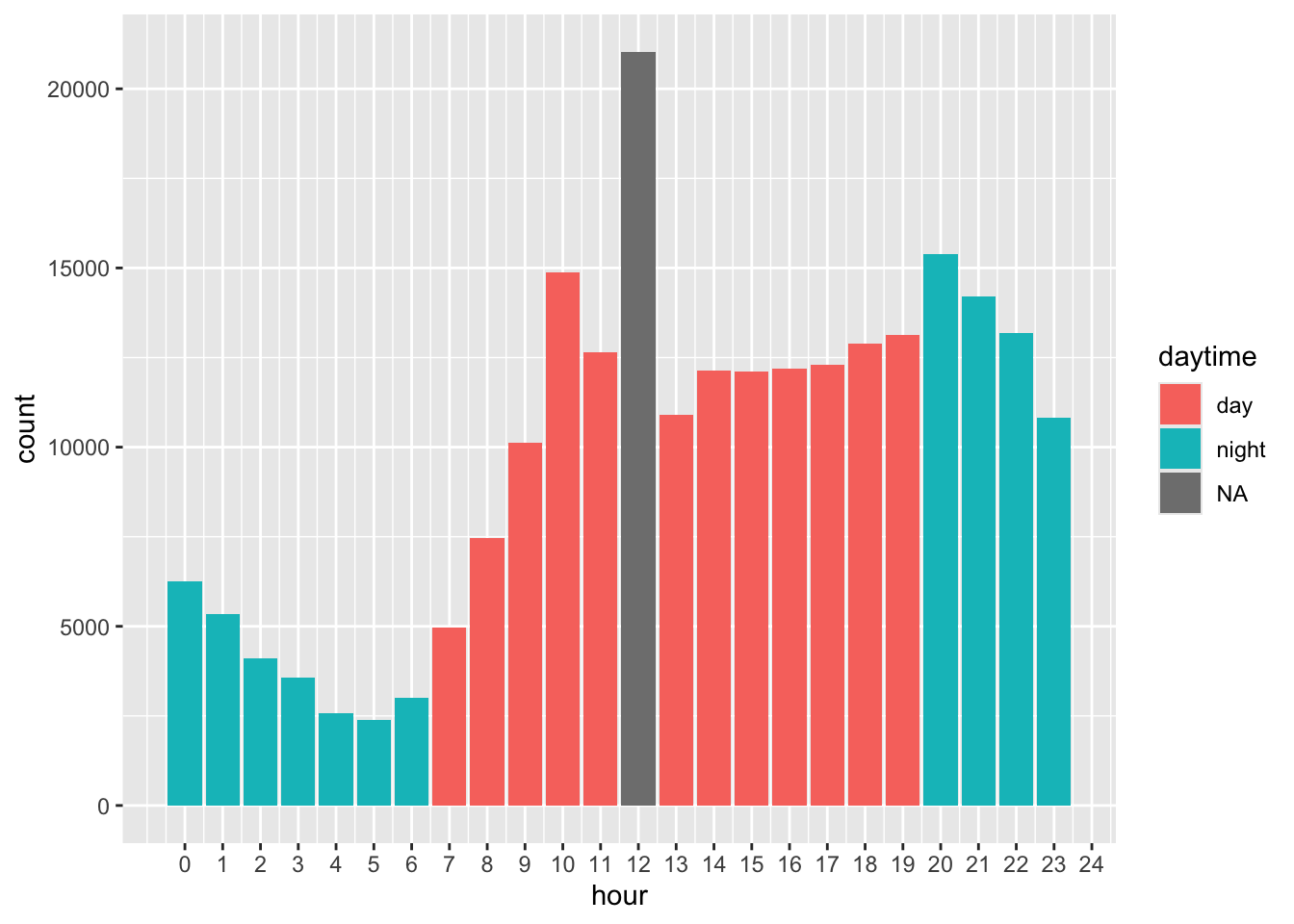
#Count the calls per day and per colonia and per night vs day
count_reports <- reports %>%
  filter(delito_lumped == "Domestic violence") %>%
  group_by(ageb, date, daytime) %>%
  filter(hour != 12) %>%
  summarise(reports_daytime = n(), .groups = "drop") %>%
  pivot_wider(names_from = daytime,
              values_from = reports_daytime,
              names_prefix = "reports_dv_",
              names_expand = T,
              values_fill = 0) %>%
  full_join(count_reports, by = c("date", "ageb"))
Count by hour of the day
Count the DV crimes per bins of two hours. I also exclude hour 12 (so only hour 13 is in that bin). Even if the count is lower than it should, it doesnt matter because were comparing this bin with the same bin another day, and NOT this bin with other bins.
#create hour_bins
reports <- reports %>%
  mutate(hour_bins = cut_width(hour, width = 2, center = 1, closed = "left"))

#Count the reports per day and per neighborhood and per bin_hour
count_reports <- reports %>%
  filter(delito_lumped == "Domestic violence") %>%
  filter(hour != 12) %>%
  group_by(date, ageb, hour_bins) %>%
  summarise(hourly_crimes = n(), .groups = "drop") %>%
  pivot_wider(names_from = hour_bins,
              values_from = hourly_crimes,
              names_prefix = "reports_dv_h",
              names_expand = T,
              values_fill = 0) %>%
  full_join(count_reports)
Count by delay in reporting
I want to count the number of crimes by category, i.e. those that were reported quickly, those that were reported with a one week delay, etc…
I have two variables for delay, that I computed earlier: - delay_full_days for the whole dataset - delay_hours only for second half of 2022 onwards (because data wasnt registered before)
First, categorize the delays in different categories for delays full days:
reports %>% count(delay_full_days) %>%
head(10) %>% kable()| delay_full_days | n |
|---|---|
| 0 | 684322 |
| 1 | 351604 |
| 2 | 123152 |
| 3 | 79534 |
| 4 | 54805 |
| 5 | 40159 |
| 6 | 32361 |
| 7 | 27112 |
| 8 | 20912 |
| 9 | 17552 |
reports <- reports %>%
  arrange(delay_full_days) %>%
  mutate(delay_category_full_days = case_when(
    delay_full_days ==  0 ~ "[0]",
    delay_full_days == 1 ~ "[1]",
    delay_full_days %in% 2:7 ~ "[2-7]",
    delay_full_days %in% 7:14 ~ "[7-14]",
    delay_full_days > 14 ~ "(14-)"),
    delay_category_full_days = as_factor(delay_category_full_days))

reports %>% count(delay_category_full_days) %>%
  filter(!is.na(delay_category_full_days)) %>%
  mutate(freq = scales::percent(n/sum(n), accuracy = .01)) %>%
kable()| delay_category_full_days | n | freq |
|---|---|---|
| [0] | 684322 | 36.43% |
| [1] | 351604 | 18.72% |
| [2-7] | 357123 | 19.01% |
| [7-14] | 103347 | 5.50% |
| (14-) | 382240 | 20.35% |
Second, categorize the delays in different categories, for delays in hours:
We can do the same for a subsample of the data, at a finer hourly measure. - Very short delays: 0-6 hours. - Short delays: 6-24 hours. - Medium delays: 24-48 hours. - Long delays: 48+ hours.
reports <- reports %>%
  arrange(delay_hours) %>%
  mutate(delay_category_hours = case_when(
    delay_hours <= 6 ~ "[0-6]",
    delay_hours > 6 & delay_hours <= 24 ~ "(6-24]",
    delay_hours > 24 & delay_hours <= 48 ~ "(24-48]",
    delay_hours > 48 & delay_hours <= 168 ~ "(48-168]",
    delay_hours > 168 ~ "(168-)"),
    delay_category_hours = as_factor(delay_category_hours))

reports %>% count(delay_category_hours) %>%
  filter(!is.na(delay_category_hours)) %>%
  mutate(freq = scales::percent(n/sum(n), accuracy = .01)) %>%
kable()| delay_category_hours | n | freq |
|---|---|---|
| [0-6] | 119949 | 24.50% |
| (6-24] | 83304 | 17.01% |
| (24-48] | 55882 | 11.41% |
| (48-168] | 84080 | 17.17% |
| (168-) | 146421 | 29.90% |
Now we can count the crimes per category of delay
#Count the calls per day and per colonia and per category of delay in full days
count_reports <- reports %>%
  filter(delito_lumped == "Domestic violence") %>%
  group_by(ageb, date, delay_category_full_days) %>%
  summarise(nr_reports_cat = n(), .groups = "drop") %>%
  pivot_wider(names_from = delay_category_full_days,
              values_from = nr_reports_cat,
              names_prefix = "reports_dv_delay_days_",
              names_expand = T,
              values_fill = 0) %>%
  full_join(count_reports, by = c("date", "ageb"))

#Count the calls per day and per colonia and per category of delay in continuous time days
count_reports <- reports %>%
  filter(delito_lumped == "Domestic violence") %>%
  filter(!is.na(delay_category_hours)) %>%
  group_by(ageb, date, delay_category_hours) %>%
  summarise(nr_reports_cat = n(), .groups = "drop") %>%
  pivot_wider(names_from = delay_category_hours,
              values_from = nr_reports_cat,
              names_prefix = "reports_dv_delay_hours_",
              names_expand = T,
              values_fill = 0) %>%
  full_join(count_reports, by = c("date", "ageb"))
Clean the counts and join
Now, crucially, we need to assign 0 for days x AGEB that got count 0 in any of those counts.
First, we need to make the dataset complete i.e. each combination of ageb x day
count_reports <- count_reports %>%
  complete(date = seq.Date(min(date), max(date), by = "day"),
           ageb = unique(ageb))
Then, we need to replace all the NAs that result (i) from the full_joins (ii) and from the complete with a count of 0.
count_reports <- count_reports %>%
  mutate(across(contains("reports"), ~ replace_na(.x, 0))) %>%
  arrange(ageb, date)
Reorder the columns for better readability.
count_reports <- count_reports %>%
  relocate(date, ageb, reports_dv, reports_dv_day, reports_dv_night, reports_all) %>%
  relocate(contains("reports_dv_delay"), contains("reports_dv_h"), .after = last_col())

names(count_reports)
[1] "date" "ageb"
[3] "reports_dv" "reports_dv_day"
[5] "reports_dv_night" "reports_all"
[7] "reports_drugs" "reports_feminicide"
[9] "reports_fraud" "reports_homicide"
[11] "reports_rapes" "reports_sexual"
[13] "reports_suicide" "reports_theft"
[15] "reports_threats" "reports_trust"
[17] "reports_other" "reports_dv_delay_hours_[0-6]"
[19] "reports_dv_delay_hours_(6-24]" "reports_dv_delay_hours_(24-48]"
[21] "reports_dv_delay_hours_(48-168]" "reports_dv_delay_hours_(168-)"
[23] "reports_dv_delay_days_[0]" "reports_dv_delay_days_[1]"
[25] "reports_dv_delay_days_[2-7]" "reports_dv_delay_days_[7-14]"
[27] "reports_dv_delay_days_(14-)" "reports_dv_h[0,2)"
[29] "reports_dv_h[2,4)" "reports_dv_h[4,6)"
[31] "reports_dv_h[6,8)" "reports_dv_h[8,10)"
[33] "reports_dv_h[10,12)" "reports_dv_h[12,14)"
[35] "reports_dv_h[14,16)" "reports_dv_h[16,18)"
[37] "reports_dv_h[18,20)" "reports_dv_h[20,22)"
[39] "reports_dv_h[22,24]" Join time and count of reports
We add the time dimensions to the count of reports.
count_reports <- count_reports %>%
  left_join(time, by = "date") %>%
  relocate(contains("reports_"), .after = last_col())

rm(reports)
Calls
Now, we do the same type of counting, but for calls. Here, we count at day x neighborhood level.
# create a combined version of location
calls <- calls %>%
  mutate(col_id = ifelse(!is.na(col_id_hechos),
                                  col_id_hechos,
                                  col_id_usuaria)) %>%
  relocate(col_id, .after = "col_id_usuaria")

# remove those that connot be located
calls <- calls %>%
  filter(!is.na(col_id))
Count all calls
Count calls per day and per neighborhood. I still have two locations: col_id_hechos and col_id_usuaria. I count for each, and for a combined version of each.
count_calls <- calls %>%
  group_by(date, col_id) %>%
  summarise(calls = n())

# using the incident location, when available
count_calls <- calls %>%
  summarise(calls_hechos = n(), .by  = c("col_id_hechos", "date")) %>%
  rename(col_id = col_id_hechos) %>%
  right_join(count_calls)

# using the caller's location, much more frequent but not precise
count_calls <- calls %>%
  summarise(calls_usuaria = n(), .by  = c("col_id_usuaria", "date")) %>%
  rename(col_id = col_id_usuaria) %>%
  right_join(count_calls)
Count at day and night
Count calls during the day and during the night. Day is 7am to 7pm included. Here we keep 12:00, because it is not mismeasured since it is recorded automatically.
#create daytime vs nighttime
calls <- calls %>%
  mutate(daytime = if_else(hour %in% 7:19, "day", "night"))

calls %>%
  ggplot(aes(x = hour, fill = daytime)) +
  geom_bar() +
  scale_x_continuous(breaks = seq(0, 24, 1))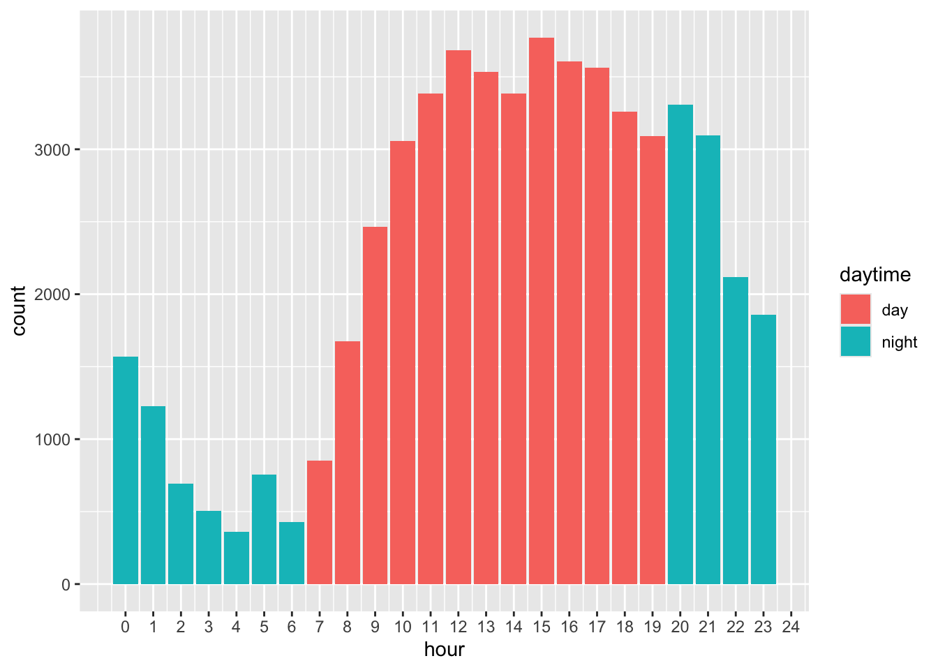
#Count the calls per day and per municipality and per night vs day
count_calls <- calls %>%
  group_by(col_id, date, daytime) %>%
  summarise(calls_daytime = n(), .groups = "drop") %>%
  pivot_wider(names_from = daytime,
              values_from = calls_daytime,
              names_prefix = "calls_",
              names_expand = T,
              values_fill = 0) %>%
  right_join(count_calls)
Count by type of DV calls
I also want to count the calls for each type when I know it;
calls %>%
  count(TYPE) %>%
  mutate(freq = scales::percent(n/sum(n))) %>%
kable()| TYPE | n | freq |
|---|---|---|
| intimate partner violence | 13376 | 24.21% |
| unknown | 13555 | 24.53% |
| violence against adult | 18879 | 34.17% |
| violence against children | 5871 | 10.63% |
| violence committed by family members | 3570 | 6.46% |
count_calls <- calls %>%
  group_by(date, col_id, TYPE) %>%
  summarise(reports = n(), .groups = "drop") %>%
  pivot_wider(names_from = TYPE,
              values_from = reports,
              names_prefix = "calls_",
              names_expand = T,
              values_fill = 0) %>%
  full_join(count_calls)
Clean the counts and join
Now, crucially, we need to assign 0 for days x AGEB that got count 0 in any of those counts.
First, we need to make the dataset complete i.e. each combination of ageb x day
count_calls <- count_calls %>%
  complete(date = seq.Date(min(date), max(date), by = "day"),
           col_id = unique(col_id))
Then, we need to replace all the NAs that result (i) from the full_joins (ii) and from the complete with a count of 0.
count_calls <- count_calls %>%
  mutate(across(contains("calls"), ~ replace_na(.x, 0))) %>%
  arrange(col_id, date)
Reorder the columns for better readability.
count_calls <- count_calls %>%
  relocate(date, col_id, calls, calls_hechos, calls_usuaria, calls_day, calls_night)

names(count_calls)
[1] "date"
[2] "col_id"
[3] "calls"
[4] "calls_hechos"
[5] "calls_usuaria"
[6] "calls_day"
[7] "calls_night"
[8] "calls_intimate partner violence"
[9] "calls_unknown"
[10] "calls_violence against adult"
[11] "calls_violence against children"
[12] "calls_violence committed by family members"Join time and count of reports
We add the time dimensions to the count of reports.
count_calls <- count_calls %>%
  left_join(time, by = "date") %>%
  relocate(contains("calls_"), .after = last_col())

rm(calls)
Create bins and assign weather and pollution
We want to add the weather variables. First, I compute some bins at the day level.
Create the bins for temperature
source(here("fun_dynamic_bins.R"))I create bins for temperature. I define a function that dynamically creates bins as a function of how many observations fall in each bin. It lumps together the extreme bins that have less than a certain proportion of observations. The rule is that the extreme bin must contain at least 1pc of observations for the 2 degree wide, and 0.5pc for the 1 degree wide.
#2 degree wide
weather <- weather %>%
  mutate(bins_temp_two = create_dynamic_bins(temp, 2, threshold_percentage = 0.01),
         bins_tmean_two = create_dynamic_bins(tmean, 2, threshold_percentage = 0.01),
         bins_tmax_two = create_dynamic_bins(tmax, 2, threshold_percentage = 0.01),
         bins_tmin_two = create_dynamic_bins(tmin, 2, threshold_percentage = 0.01))

#and 1 degree wide
weather <- weather %>%
  mutate(bins_temp_one = create_dynamic_bins(temp, 1, threshold_percentage = 0.005),
         bins_tmean_one = create_dynamic_bins(tmean, 1, threshold_percentage = 0.005),
         bins_tmax_one = create_dynamic_bins(tmax, 1, threshold_percentage = 0.005),
         bins_tmin_one = create_dynamic_bins(tmin, 1, threshold_percentage = 0.005))
weather %>%
group_by(year) %>%
summarise(total = n(),
missing_tmean = sum(is.na(tmean))) %>%
mutate(share = scales::percent(missing_tmean/total)) %>%
kable()| year | total | missing_tmean | share |
|---|---|---|---|
| 2016 | 889746 | 1 | 0.00011% |
| 2017 | 887315 | 30 | 0.00338% |
| 2018 | 887315 | 3 | 0.00034% |
| 2019 | 887315 | 27 | 0.00304% |
| 2020 | 889746 | 129 | 0.01450% |
| 2021 | 887315 | 108 | 0.01217% |
| 2022 | 887315 | 35 | 0.00394% |
| 2023 | 887315 | 0 | 0.00000% |
| 2024 | 889746 | 299059 | 33.61173% |
| 2025 | 136136 | 136136 | 100.00000% |
weather %>%
  count(bins_tmean_one, bins_tmean_two) %>%
  drop_na() %>%
  mutate(prop_in_pc = scales::percent(n / sum(n))) %>%
kable()| bins_tmean_one | bins_tmean_two | n | prop_in_pc |
|---|---|---|---|
| <11 | <12 | 68135 | 0.886% |
| [11,12) | <12 | 83380 | 1.084% |
| [12,13) | [12,14) | 178142 | 2.315% |
| [13,14) | [12,14) | 322396 | 4.190% |
| [14,15) | [14,16) | 544411 | 7.076% |
| [15,16) | [14,16) | 879383 | 11.430% |
| [16,17) | [16,18) | 1144938 | 14.881% |
| [17,18) | [16,18) | 1329697 | 17.283% |
| [18,19) | [18,20) | 1190293 | 15.471% |
| [19,20) | [18,20) | 848028 | 11.022% |
| [20,21) | [20,22) | 524100 | 6.812% |
| [21,22) | [20,22) | 326046 | 4.238% |
| [22,23) | >=22 | 151589 | 1.970% |
| >=23 | >=22 | 103198 | 1.341% |
Join weather to the count of reports
Straightforward, since both are day per ageb level.
Weather is missing for some days x ageb, but very few in general.
data_reports <- count_reports %>%
  left_join(weather)

data_reports %>%
  group_by(year) %>%
  summarise(total = n(),
            missing_tmean = sum(is.na(tmean))) %>%
  mutate(share = scales::percent(missing_tmean/total)) %>%
kable()| year | total | missing_tmean | share |
|---|---|---|---|
| 2016 | 889014 | 1 | 0.00011% |
| 2017 | 886585 | 30 | 0.00338% |
| 2018 | 886585 | 3 | 0.00034% |
| 2019 | 886585 | 27 | 0.00305% |
| 2020 | 889014 | 129 | 0.01451% |
| 2021 | 886585 | 108 | 0.01218% |
| 2022 | 886585 | 35 | 0.00395% |
| 2023 | 886585 | 0 | 0.00000% |
| 2024 | 592676 | 2475 | 0.41760% |
Join weather to the count of calls
Less straightforward, since weather is measured at AGEB level. I could compute weather all over again at the neighborhood level, but since the scale is so tiny, I will just assign the weather of the AGEB to the neighborhood.
Match AGEBs and colonias
First, establish a correspondance between AGEB and neighborhoods.
poligonos %>% distinct(ageb) %>% nrow()[1] 2431colonias %>% distinct(col_id) %>% nrow()[1] 1948# Compute centroids
colonias_centroids <- colonias %>% select(col_id) %>% st_centroid()
agebs_centroids <- poligonos %>% select(ageb) %>% st_centroid()
colonias_nearest_ageb <-
st_join(colonias_centroids, agebs_centroids, join = st_nearest_feature) %>%
select(col_id, ageb) %>%
st_drop_geometry()We can plot the connections, just for fun, but exactly what we expected.
connections <- colonias_nearest_ageb %>%
  left_join(colonias_centroids, by = "col_id") %>%
  left_join(agebs_centroids, by = "ageb") %>%
#   Convert each pair of points into a LINESTRING
  rowwise() %>%
  mutate(geometry = st_sfc(st_linestring(rbind(st_coordinates(geom),
                                               st_coordinates(geometry))),
                           crs = 4326)) %>%
  ungroup() %>%
  select(col_id, ageb, geometry) %>%
  st_as_sf()

ggplot() +
  geom_sf(data = colonias_centroids, size = .2, color = "red", alpha = .5) +
  #geom_sf(data = agebs_centroids, size = .2, color = "red", alpha = .5) +
  geom_sf(data = connections, color = "blue", alpha = 1) +
  labs(title = "Connections between colonias and AGEBs centroids") +
  theme_light() +
annotation_scale(location = "br", style = "ticks") 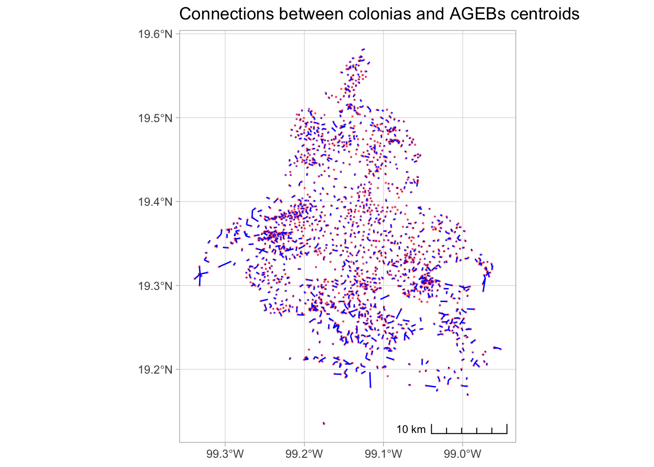
Actually join the data
We assign to each neighborhood the identifier of the closest AGEB.
count_calls <- count_calls %>%
  left_join(colonias_nearest_ageb)
And based on this AGEB, we can merge the weather data.
data_calls <- count_calls %>%
  left_join(weather)

# remove the ageb identifier, it was just for the join
# do not get confused
data_calls <- data_calls %>% select(-ageb)
There are only very few missing temp obs.
data_calls %>%
  group_by(year) %>%
  summarise(total = n(),
            missing_tmean = sum(is.na(tmean))) %>%
  mutate(share = scales::percent(missing_tmean/total)) %>%
kable()| year | total | missing_tmean | share |
|---|---|---|---|
| 2016 | 84180 | 0 | 0.00000% |
| 2017 | 503700 | 24 | 0.00476% |
| 2018 | 503700 | 2 | 0.00040% |
| 2019 | 503700 | 27 | 0.00536% |
| 2020 | 505080 | 93 | 0.01841% |
| 2021 | 503700 | 105 | 0.02085% |
| 2022 | 335340 | 6 | 0.00179% |
Save the final datasets
We save one dataset for reports and another for calls since they’re on different levels.
Reports is AGEB per day, calls is neighborhood per day.
data_reports <- data_reports %>%
  mutate(year = as_factor(year)) %>%
  relocate(starts_with("bins"),
           starts_with("reports"),
           .after = last_col()) %>%
  relocate(ageb, date,
           reports_dv,
           tmean, bins_tmean_one, prec, tmax, tmin, pm25_mean) %>%
  # remove temp = tmin+tmax/2, we now use tmean, the 24 hourly avg
  select(-contains("temp"))


data_reports %>%
  select( - tmp_hourly) %>%
  write_rds(here("..", "output",
                 "data_reports.rds"))

# save the hourly list separately, its just very big
data_reports %>%
  select(date, ageb, tmp_hourly) %>%
  write_rds(here("..", "output", "temporary_data",
                 "tmp_hourly_ageb.rds"))
data_calls <- data_calls %>%
mutate(year = as_factor(year)) %>%
relocate(starts_with("bins"),
starts_with("calls"),
.after = last_col()) %>%
relocate(col_id, date,
calls,
tmean, bins_tmean_one, prec, tmax, tmin, pm25_mean) %>%
# remove temp = tmin+tmax/2, we now use tmean, the 24 hourly avg
select(-contains("temp"))
data_calls %>%
select( - tmp_hourly) %>%
write_rds(here("..", "output",
"data_calls.rds"))
data_calls %>%
select(date, col_id, tmp_hourly) %>%
write_rds(here("..", "output", "temporary_data",
"tmp_hourly_col_id.rds"))