Heterogeneity: income

Note

I run the heterogeneity on income.

I interact with above/below median, quintiles and deciles.

I save a plot for bins and above/below median
I save a table for linear quintiles
I save two plots for bins and quintiles

Generally, the quintiles is much more interesting than the above/below median

There is a clear gradient in the quintiles in the linear reg From 3.1% for the poorest to 2% for the richest with the bins, its hard to see, comparing dozens of coefficients

So i do bins and above below median. The linear is not very striking I get 2.9% for the poor, 2.4% for the rich However, with the bins, there is a small difference in “slope” which is kind of interesting

So probably the best is to show the table for quintiles and the plots for the above/below median with the bins

start_time <- Sys.time()

library(tidyverse)
library(here) # path control
library(fixest) # estimations with fixed effects
library(knitr)
library(sf)
library(tictoc)
tic("Total render time")

source("fun_dynamic_bins.R")
source("fixest_etable_options.R")

data <-
  read_rds(here("..", "output", "data_reports.rds")) %>% 
  filter(covid_phase == "Pre-pandemic")

data <- data %>% 
  mutate(prec_quintile = ntile(prec, 5),
         rh_quintile = ntile(rh, 5),
         wsp_quintile = ntile(wsp, 5))

ageb_attributes <- 
  readRDS(here("..", "output", "ageb_attributes.rds"))

poligonos <-  
  read_sf(here("..",
                "output",
                "ageb_poligonos.geojson"),
          quiet = TRUE)

Compute ntiles for income

I bin AGEBs into income deciles, quintiles and above/below median. I weight by population so that there are the same number of ppl in each decile and not the same number of AGEBs.

ageb_attributes <- ageb_attributes %>% 
  arrange(income) %>% 
  mutate(
    # Population-Weighted Deciles
    income_decile = ifelse(
      is.na(income) | is.na(pobtot), NA, 
      as_factor(cut(
        cumsum(pobtot[!is.na(income)]) / sum(pobtot[!is.na(income)], na.rm = TRUE), 
        breaks = seq(0, 1, by = 0.1), 
        labels = 1:10, 
        include.lowest = TRUE
      ))
    )) %>% 
  mutate(
    income_quintile = case_when(
      income_decile %in% c("1", "2") ~ "1",
      income_decile %in% c("3", "4") ~ "2",
      income_decile %in% c("5", "6") ~ "3",
      income_decile %in% c("7", "8") ~ "4",
      income_decile %in% c("9", "10") ~ "5",
      TRUE ~ NA),
    income_median = case_when(
      income_decile %in% c("1", "2", "3", "4", "5") ~ "Below Median",
      income_decile %in% c("6", "7", "8", "9", "10") ~ "Above Median",
      TRUE ~ NA)
  ) %>% 
  mutate(
    income_decile = as_factor(income_decile),
    income_quintile = as_factor(income_quintile),
    income_median = as_factor(income_median)
  )

Visualize income quintiles:

ageb_attributes %>% 
  ggplot(aes(x = income_decile, y = income, color = income_quintile)) +
  geom_boxplot() +
  labs(title = "Income distribution within deciles (ageb level)",
       x = "Income Decile", y = "Income",) +
  guides(color = "none") +
  theme_light()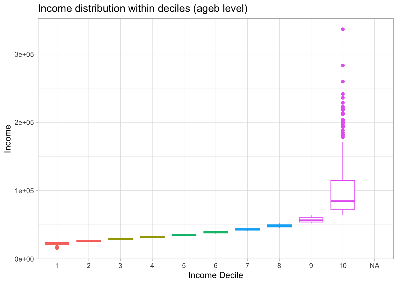

full_join(poligonos, ageb_attributes) %>% 
  ggplot() +
  geom_sf(aes(fill = income_quintile), color = NA) +
  scale_fill_brewer(palette = "RdYlBu", direction = 1, na.value = "grey90") +
  labs(title = "Income Quintiles by AGEB", fill = "Quintile") +
  theme_light()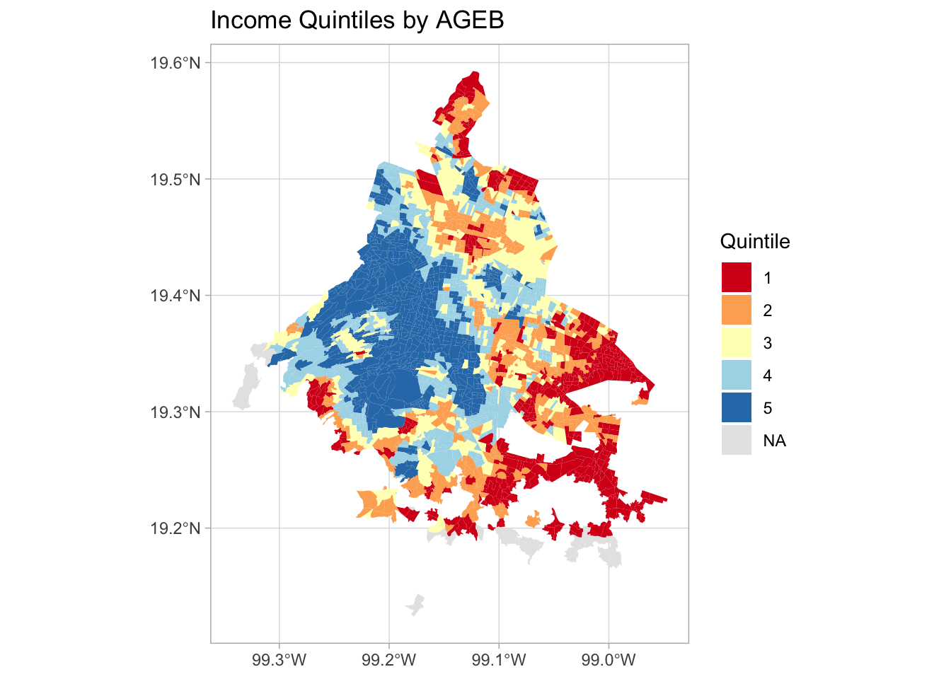

ageb_attributes %>%
  filter(!is.na(income_quintile)) %>%
  group_by(income_quintile) %>%
  summarise(
    mean_income = mean(income, na.rm = TRUE),
    pobtot = sum(pobtot, na.rm = TRUE)
    ) %>%
  kable()

income_quintile	mean_income	pobtot
1	24511.90	1802283
2	30623.98	1802272
3	37101.17	1798938
4	45775.35	1804070
5	80920.06	1805085

Join these ageb attributes to the main panel:

# Merge with data
data <- 
  left_join(data, ageb_attributes)

Average level of crime per income quintile:

data %>%
  # filter(!is.na(income_quintile)) %>%
  group_by(income_quintile) %>%
  summarise(
    mean_reports = mean(reports_dv, na.rm = TRUE),
    total_reports = sum(reports_dv, na.rm = TRUE)
  ) %>%
  kable()

income_quintile	mean_reports	total_reports
1	0.0249909	15318
2	0.0281556	18233
3	0.0246617	17976
4	0.0234682	17000
5	0.0162459	14533
NA	0.0232806	1157

Baseline regressions for reference

First the baseline regressions for reference:

baseline_linear <- data %>% 
  fepois(reports_dv ~ tmean |
           prec_quintile + rh_quintile + wsp_quintile +
           ageb + year^month + day_of_week + day_of_year,
         cluster = ~ ageb)

baseline_bins <- data %>% 
  mutate(bins_tmean_one = create_dynamic_bins(tmean, width = 1, 0.01)) %>% 
  fepois(reports_dv ~ i(bins_tmean_one, ref = "[16") |
           prec_quintile + rh_quintile + wsp_quintile +
           ageb + year^month + day_of_week + day_of_year,
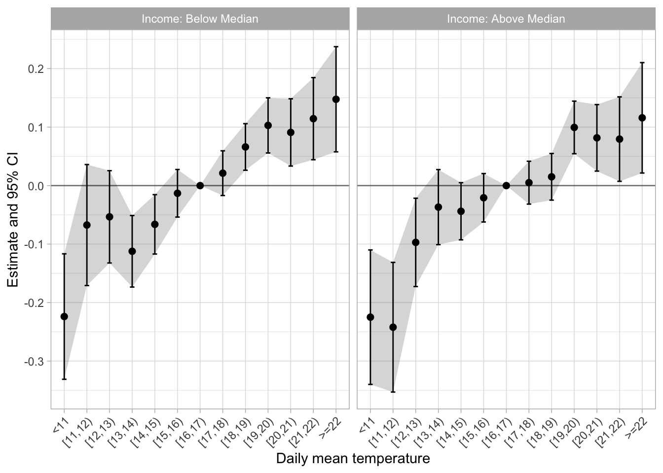
         cluster = ~ ageb)

Above/below median income

I can also do simple categories; above and below median.

Imposing linearity, its only two estimates, I don’t export the table

reg_above_below_linear <- data %>%
  fepois(reports_dv ~ i(income_median, tmean) |
           prec_quintile + rh_quintile + wsp_quintile +
           ageb + year^month + day_of_week + day_of_year,
         cluster = ~ ageb)

etable(baseline_linear, reg_above_below_linear) %>% 
  kable()

	baseline_linear	reg_above_below_..
Dependent Var.:	Reports for DV	Reports for DV

Temperature	0.0274*** (0.0034)
Temperature x income_median = BelowMedian		0.0289*** (0.0037)
Temperature x income_median = AboveMedian		0.0251*** (0.0038)
Fixed-Effects:	——————	——————
Prec, hum, wsp quintiles	Yes	Yes
Neighborhood	Yes	Yes
Year-Month	Yes	Yes
Day of Week	Yes	Yes
Day of Year	Yes	Yes
________________________________________	__________________	__________________
S.E.: Clustered	by: Neighborhood	by: Neighborhood
Observations	3,624,826	3,578,253

Or semi parametric with bins:

reg_above_below_bins <- data %>%
  mutate(bins_tmean_one = create_dynamic_bins(tmean, width = 1, 0.01)) %>% 
  fepois(reports_dv ~ i(income_median, bins_tmean_one, ref2 = "[16") |
           prec_quintile + rh_quintile + wsp_quintile +
           ageb + year^month + day_of_week + day_of_year,
         cluster = ~ ageb)

I can plot these results and save as reg_income_median.png

Income quintile regressions

I first run the model imposing linearity on tmean and interacting it with income quintiles.

reg_quintile_linear <- data %>%
  fepois(reports_dv ~ i(income_quintile, tmean) |
           prec_quintile + rh_quintile + wsp_quintile +
           ageb + year^month + day_of_week + day_of_year,
         cluster = ~ ageb)

etable(reg_quintile_linear) %>% 
  kable()

	reg_quintile_lin..
Dependent Var.:	Reports for DV

Temperature x income_quintile = 1	0.0342*** (0.0048)
Temperature x income_quintile = 2	0.0297*** (0.0044)
Temperature x income_quintile = 3	0.0254*** (0.0045)
Temperature x income_quintile = 4	0.0239*** (0.0046)
Temperature x income_quintile = 5	0.0216*** (0.0048)
Fixed-Effects:	——————
Prec, hum, wsp quintiles	Yes
Neighborhood	Yes
Year-Month	Yes
Day of Week	Yes
Day of Year	Yes
_________________________________	__________________
S.E.: Clustered	by: Neighborhood
Observations	3,578,253

Export the table as reg_income_quintile.tex

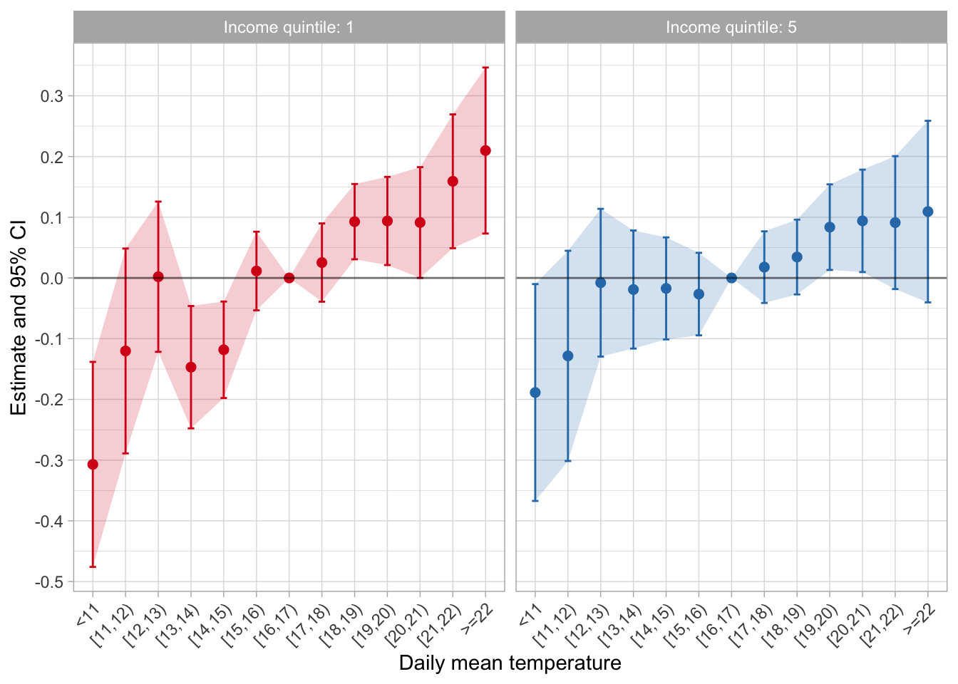
I then allow for possible non-linearities in the relationship between temperature and DV. With the quintiles, its a bit of a crazy estimation…

tic("quintile")
reg_quintile_bins <- data %>%
  mutate(bins_tmean_one = create_dynamic_bins(tmean, width = 1, 0.01)) %>% 
  fepois(reports_dv ~ i(income_quintile, bins_tmean_one, ref2 = "[16") |
           prec_quintile + rh_quintile + wsp_quintile +
           ageb + year^month + day_of_week + day_of_year,
         cluster = ~ ageb)
toc()

quintile: 2423.325 sec elapsed

I plot these results.

I save the full results as reg_income_quintiles_bins_full.png.

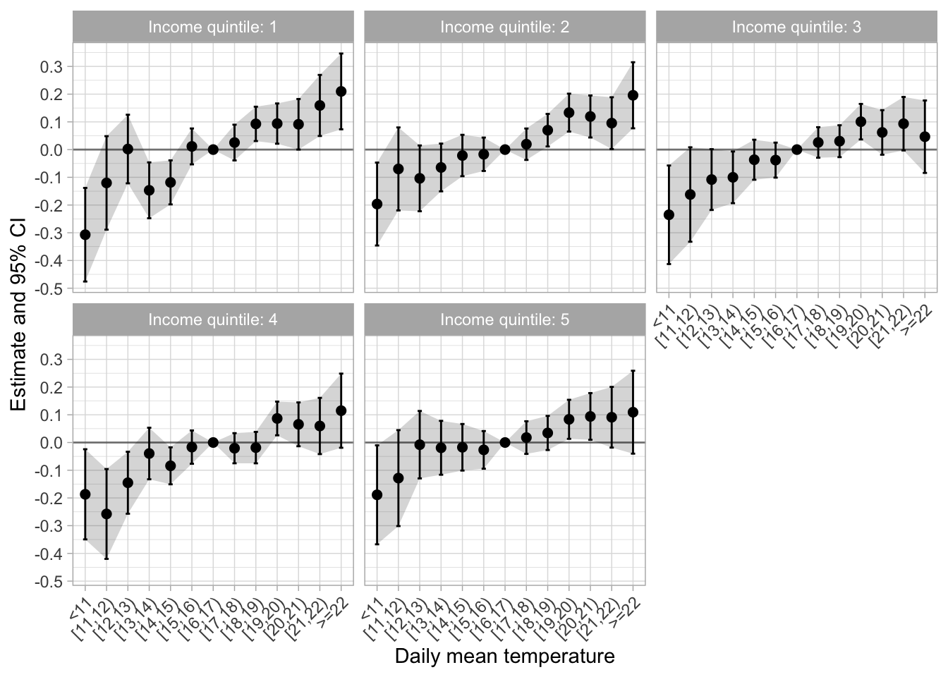
And only the two extreme quintiles as reg_income_quintiles_bins_extreme.png

Income decile

I also tried using decile instead of quintile, but it doesnt add much else than noise and it takes too long to run.

tic("decile")
reg_decile_linear <- data %>%
  fepois(reports_dv ~ i(income_decile, tmean) |
           prec_quintile + rh_quintile + wsp_quintile +
           ageb + year^month + day_of_week + day_of_year,
         cluster = ~ ageb)
toc()

decile: 194.053 sec elapsed

etable(reg_decile_linear) %>% 
  kable()

	reg_decile_linear
Dependent Var.:	Reports for DV

Temperature x income_decile = 1	0.0377*** (0.0063)
Temperature x income_decile = 2	0.0314*** (0.0059)
Temperature x income_decile = 3	0.0263*** (0.0057)
Temperature x income_decile = 4	0.0332*** (0.0053)
Temperature x income_decile = 5	0.0182** (0.0058)
Temperature x income_decile = 6	0.0328*** (0.0054)
Temperature x income_decile = 7	0.0233*** (0.0057)
Temperature x income_decile = 8	0.0245*** (0.0059)
Temperature x income_decile = 9	0.0198*** (0.0058)
Temperature x income_decile = 10	0.0237*** (0.0063)
Fixed-Effects:	——————
Prec, hum, wsp quintiles	Yes
Neighborhood	Yes
Year-Month	Yes
Day of Week	Yes
Day of Year	Yes
________________________________	__________________
S.E.: Clustered	by: Neighborhood
Observations	3,578,253

Rendered on: 2025-07-27 03:01:11

Total render time: 3397.264 sec elapsed