all_files <-
  # get full path
  tibble(path = list.files(here("..", "raw_data", "3_aire_cdmx", "EXCEL_new"),
                           pattern = ".*xls$",
                           recursive = T,
                           full.names = T)) %>%
  mutate(basename = tools::file_path_sans_ext(basename(path)),
         year_file = as.numeric(str_sub(basename, 1, 4)),
         variable = str_sub(basename, 5),
         source = str_extract(path, "(?<=EXCEL_new/)[^/]+")) %>%
filter(source == "RAMA")Pollution data from RAMA
Note
In this script, I wrangle the pollution data. I downloaded it from aire.cdmx.gob.mx in EXCEL format. The updated data was sent to me by email because their site went down. The source that measures at the station by hour level for Mexico City is RAMA (Red Automática de Monitoreo Atmosférico) for CO, NO, NO2, NOX, 03, PM10, PM25, PMCO, SO2.
Warning
Warning: Script is heavy, relies on parallelization, takes a couple hours to run.
Some parameters: - I remove a measured day if more than 4 hours out of 24 are missing - Inverse distance weight within 20km
Import RAMA hourly data
First, list all the excel files.
Import all the data and join into a single dataframe.
# import all the data in lists
hourly_data <-
  map(all_files %>% pull(variable) %>% unique(), ~{
    print(paste0("Importing: ", .x))

    all_files %>%
      filter(variable == .x) %>%
      pull(path) %>%
      map(~ read_xls(.)) %>%
      list_rbind() %>%
      pivot_longer(cols = -c(FECHA, HORA),
                   names_to = "station",
                   values_to = .x)
  }, .progress = TRUE)
[1] "Importing: CO"
[1] "Importing: NO"[1] "Importing: NO2"[1] "Importing: NOX"
[1] "Importing: O3"[1] "Importing: PM10"
[1] "Importing: PM25"[1] "Importing: PMCO"
[1] "Importing: SO2"#reduce the lists by dataset
hourly_data <- hourly_data %>%
reduce(full_join, by = c("FECHA", "HORA", "station"))
#rename and encode
hourly_data <- hourly_data %>%
rename_with(tolower) %>%
mutate(fecha = as_date(fecha))
rm(all_files)Distances between stations and AGEBs
Location of all the stations
catalogo_est <-
  read_csv(here("..",
                "raw_data",
                "3_aire_cdmx",
                "cat_estacion.csv"),
           skip = 1,
           locale = readr::locale(encoding = "latin1")) %>%
  rename(station = cve_estac)

# all the stations are in the catalog
catalogo_est <- catalogo_est %>%
  filter(station %in% (hourly_data %>% pull(station) %>% unique()))
Locations of the AGEB
catalogo_ageb <-
  read_sf(here("..",
                "output",
                "ageb_poligonos.geojson"),
          quiet = TRUE) %>%
  st_transform(4326)

catalogo_ageb <- catalogo_ageb %>%
  st_centroid() %>%
  mutate(lon = st_coordinates(.)[, 1],
         lat = st_coordinates(.)[, 2]) %>%
  st_drop_geometry() %>% as_tibble()
I want to compute the distances between each station and the centroid of each AGEB.
# Compute the distances between each station and the col centroids
# create a df from all combinations of stations and municipalities
distances <-
  crossing(
    (catalogo_ageb %>% select(ageb,
                             ageb_lon = lon,
                             ageb_lat = lat)),
    (catalogo_est %>% select(station,
                             sta_lon = longitud,
                             sta_lat = latitud))
  )

# compute the distance in meters, using haversine method, and convert to km
distances <- distances %>%
  mutate(distance = geosphere::distHaversine(cbind(ageb_lon, ageb_lat),
                                             cbind(sta_lon, sta_lat)),
         distance = distance/1000)

distances %>%
  write_rds(here("..", "output",
                 "temporary_data",
                 "weather",
                 "distances_pollution.rds"))

distances %>%
  write_rds(here("..", "output",
                 "temporary_data",
                 "weather",
                 "distances_precipitation.rds"))

#Only keep the combinations that are within 20km
distances <- distances %>%
  filter(distance <= 20)
Look at missing data in the pollution data
# encode missing variables!
hourly_data <- hourly_data %>%
  mutate(across(where(is.numeric), ~ na_if(., -99)))
Vast majority of stations have data have at some point for some variables. So we keep them all.
hourly_data %>%
  group_by(station) %>%
  summarise(across(.cols = where(is.numeric) & !hora,
                   .fns = ~ sum(is.na(.)) / n())) %>%
kable()| station | co | no | no2 | nox | o3 | pm10 | pm25 | pmco | so2 |
|---|---|---|---|---|---|---|---|---|---|
| ACO | 0.4130948 | 0.4094128 | 0.4094246 | 0.4094010 | 0.4015059 | 0.3221417 | 1.0000000 | 1.0000000 | 0.4490653 |
| AJM | 0.3233218 | 0.3032949 | 0.3032949 | 0.3032949 | 0.3000260 | 0.3974462 | 0.3974698 | 0.3974462 | 0.2730245 |
| AJU | 1.0000000 | 1.0000000 | 0.9999882 | 0.9999646 | 0.2868674 | 1.0000000 | 0.4946186 | 1.0000000 | 1.0000000 |
| ATI | 0.2333483 | 0.3177988 | 0.3177988 | 0.3177988 | 0.1943566 | 0.2376204 | 1.0000000 | 1.0000000 | 0.2468726 |
| BJU | 0.1520723 | 1.0000000 | 0.4807874 | 1.0000000 | 0.1513878 | 0.1794869 | 0.1794987 | 0.1794751 | 0.2463888 |
| CAM | 0.2389657 | 0.2297371 | 0.2297371 | 0.2297371 | 0.2085182 | 0.2996011 | 0.2996011 | 0.2996011 | 0.2577181 |
| CCA | 0.1172111 | 0.1221795 | 0.1221795 | 0.1221795 | 0.0903158 | 1.0000000 | 0.1100477 | 1.0000000 | 0.1015743 |
| CHO | 0.3887132 | 0.6429617 | 0.6429617 | 0.6429617 | 0.3432189 | 0.3688633 | 1.0000000 | 1.0000000 | 0.4135786 |
| COY | 1.0000000 | 0.7613765 | 0.7613765 | 0.7613765 | 0.7438633 | 1.0000000 | 0.7371011 | 1.0000000 | 1.0000000 |
| CUA | 0.1442952 | 0.1732912 | 0.1732912 | 0.1732912 | 0.1455580 | 0.2439459 | 1.0000000 | 1.0000000 | 0.2458577 |
| CUT | 0.8409767 | 0.1309597 | 0.1309597 | 0.1309597 | 0.1178248 | 0.1363647 | 1.0000000 | 1.0000000 | 0.1229348 |
| FAC | 0.0992376 | 0.1048197 | 0.1048197 | 0.1048197 | 0.0928413 | 0.1936721 | 1.0000000 | 1.0000000 | 0.1192763 |
| FAR | 0.5744548 | 1.0000000 | 0.4904763 | 1.0000000 | 0.5180207 | 1.0000000 | 0.5103734 | 1.0000000 | 0.5065380 |
| GAM | 1.0000000 | 1.0000000 | 0.5002596 | 1.0000000 | 0.2157643 | 0.7056623 | 0.5309314 | 0.7056623 | 1.0000000 |
| HGM | 0.3827771 | 0.3836858 | 0.3836858 | 0.3836858 | 0.3779149 | 0.4898626 | 0.4898626 | 0.4898744 | 0.3722267 |
| INN | 0.3380617 | 1.0000000 | 1.0000000 | 1.0000000 | 0.2739568 | 0.4072059 | 0.4072059 | 0.4072295 | 0.2833860 |
| IZT | 0.2094505 | 0.2171804 | 0.2171804 | 0.2171804 | 0.1990889 | 0.2762816 | 1.0000000 | 1.0000000 | 0.2339029 |
| LAA | 1.0000000 | 1.0000000 | 1.0000000 | 1.0000000 | 1.0000000 | 1.0000000 | 1.0000000 | 1.0000000 | 1.0000000 |
| LLA | 0.6706123 | 0.7467428 | 0.7467428 | 0.7467428 | 0.1929168 | 1.0000000 | 1.0000000 | 1.0000000 | 0.4798315 |
| LPR | 0.2030188 | 1.0000000 | 1.0000000 | 1.0000000 | 0.1764893 | 1.0000000 | 1.0000000 | 1.0000000 | 0.2182189 |
| MER | 0.1110154 | 0.1078762 | 0.1078762 | 0.1078762 | 0.0829754 | 0.1585395 | 0.1585395 | 0.1585395 | 0.0940096 |
| MGH | 0.0800014 | 0.1202559 | 0.1202559 | 0.1202559 | 0.0790219 | 0.5714690 | 0.5714690 | 0.5714690 | 0.1215422 |
| MON | 0.2363222 | 0.2044586 | 0.2044586 | 0.2044586 | 0.2164959 | 1.0000000 | 0.6349603 | 1.0000000 | 0.3303673 |
| MPA | 0.3881821 | 1.0000000 | 0.6100949 | 1.0000000 | 0.2928507 | 0.5930183 | 0.5930183 | 0.5930183 | 0.3097503 |
| NEZ | 0.1610059 | 0.1944038 | 0.1944038 | 0.1944038 | 0.1338864 | 0.7511447 | 0.2035380 | 1.0000000 | 0.1925864 |
| PED | 0.1498419 | 0.1429145 | 0.1429145 | 0.1429145 | 0.1301218 | 0.4462212 | 0.4462212 | 0.4462212 | 0.1384535 |
| SAC | 0.5287953 | 0.5089808 | 0.5089808 | 0.5089808 | 0.5169231 | 1.0000000 | 0.5448924 | 1.0000000 | 0.6960088 |
| SAG | 0.2102530 | 0.1710607 | 0.1710607 | 0.1710607 | 0.1600736 | 0.3222715 | 0.3222715 | 0.3222715 | 0.2844364 |
| SFE | 0.4136731 | 0.4002549 | 0.4002549 | 0.4002549 | 0.3572272 | 0.4343136 | 0.4343136 | 0.4343136 | 0.3565545 |
| SJA | 0.8049235 | 0.8322555 | 0.8320312 | 0.8320312 | 0.8065167 | 1.0000000 | 0.9337354 | 1.0000000 | 0.8034956 |
| SUR | 0.9803625 | 0.9803625 | 0.9803625 | 0.9803625 | 0.9663189 | 0.9520747 | 1.0000000 | 1.0000000 | 0.9846582 |
| TAH | 0.2696847 | 0.3297536 | 0.3297418 | 0.3297418 | 0.2386943 | 0.3592216 | 1.0000000 | 1.0000000 | 0.2691536 |
| TLA | 0.1502313 | 0.1426194 | 0.1426194 | 0.1426194 | 0.1195124 | 0.2131916 | 0.2131916 | 0.2131916 | 0.1217664 |
| TLI | 0.3835678 | 0.3681788 | 0.3681788 | 0.3681788 | 0.3733006 | 0.4794538 | 1.0000000 | 1.0000000 | 0.3769000 |
| TPN | 1.0000000 | 0.9829352 | 0.9829352 | 0.9829352 | 0.9517088 | 1.0000000 | 1.0000000 | 1.0000000 | 0.9829352 |
| UAX | 0.1469623 | 0.1341461 | 0.1341461 | 0.1341461 | 0.1146738 | 1.0000000 | 0.1874528 | 1.0000000 | 0.1471157 |
| UIZ | 0.1729253 | 0.1765601 | 0.1765601 | 0.1765601 | 0.1431151 | 0.3264020 | 0.3263902 | 0.3263902 | 0.1892112 |
| VIF | 0.1889634 | 0.1966461 | 0.1966461 | 0.1966461 | 0.1811863 | 0.2298315 | 1.0000000 | 1.0000000 | 0.1799825 |
| XAL | 0.4289676 | 0.4461740 | 0.4461740 | 0.4461740 | 0.4200812 | 0.5672796 | 0.5672796 | 0.5672796 | 0.4175911 |
We are going to look at daily averages. When doing so, it is crucial to know how many hours are missing for each day. For all variables, all 24 hours are recorded in +70% of the cases. Then, about 4% of the time, the station has some hours missing in the day.
hourly_missings <- hourly_data %>%
  group_by(fecha, station) %>%
  summarise(across(co:so2, ~ sum(is.na(.)), .names = "hours_missing_{.col}")) %>%
  mutate(across(starts_with("hours_missing"), ~ case_when(. == 0 ~ "0",
                                                          . %in% 1:4 ~ "1-4",
                                                          . %in% 5:23 ~ "5-23",
                                                          . == 24 ~ "24"),
                .names = "{.col}_fct")) %>% ungroup()

hourly_missings %>% count(hours_missing_pm25) %>% mutate(prop = n / sum(n)) %>% kable()| hours_missing_pm25 | n | prop |
|---|---|---|
| 0 | 35436 | 0.2573252 |
| 1 | 6019 | 0.0437081 |
| 2 | 2278 | 0.0165421 |
| 3 | 1911 | 0.0138771 |
| 4 | 1513 | 0.0109869 |
| 5 | 855 | 0.0062087 |
| 6 | 475 | 0.0034493 |
| 7 | 394 | 0.0028611 |
| 8 | 284 | 0.0020623 |
| 9 | 220 | 0.0015976 |
| 10 | 188 | 0.0013652 |
| 11 | 149 | 0.0010820 |
| 12 | 157 | 0.0011401 |
| 13 | 146 | 0.0010602 |
| 14 | 145 | 0.0010529 |
| 15 | 114 | 0.0008278 |
| 16 | 95 | 0.0006899 |
| 17 | 70 | 0.0005083 |
| 18 | 87 | 0.0006318 |
| 19 | 52 | 0.0003776 |
| 20 | 26 | 0.0001888 |
| 21 | 39 | 0.0002832 |
| 22 | 25 | 0.0001815 |
| 23 | 122 | 0.0008859 |
| 24 | 86909 | 0.6311062 |
hourly_missings %>% count(hours_missing_pm25_fct) %>% mutate(prop = n / sum(n)) %>% kable()| hours_missing_pm25_fct | n | prop |
|---|---|---|
| 0 | 35436 | 0.2573252 |
| 1-4 | 11721 | 0.0851143 |
| 24 | 86909 | 0.6311062 |
| 5-23 | 3643 | 0.0264543 |
hourly_missings %>% count(hours_missing_pm10_fct) %>% mutate(prop = n / sum(n)) %>% kable()| hours_missing_pm10_fct | n | prop |
|---|---|---|
| 0 | 41620 | 0.3022315 |
| 1-4 | 14505 | 0.1053308 |
| 24 | 77060 | 0.5595858 |
| 5-23 | 4524 | 0.0328519 |
hourly_missings %>% count(hours_missing_so2_fct) %>% mutate(prop = n / sum(n)) %>% kable()| hours_missing_so2_fct | n | prop |
|---|---|---|
| 0 | 58554 | 0.4252010 |
| 1-4 | 24460 | 0.1776209 |
| 24 | 51079 | 0.3709198 |
| 5-23 | 3616 | 0.0262583 |
We can plot this station recording activity:
hourly_missings %>%
  ggplot(aes(x = fecha, y = station, col = hours_missing_pm25_fct)) +
  geom_point(shape = 15) +
  scale_color_manual(values = c("0" = "green",
                                "1-4" = "blue",
                                "5-23" = "red",
                                "24" = "gray")) +
  labs(title = "Station activity for pm25") +
  theme(legend.position = "bottom")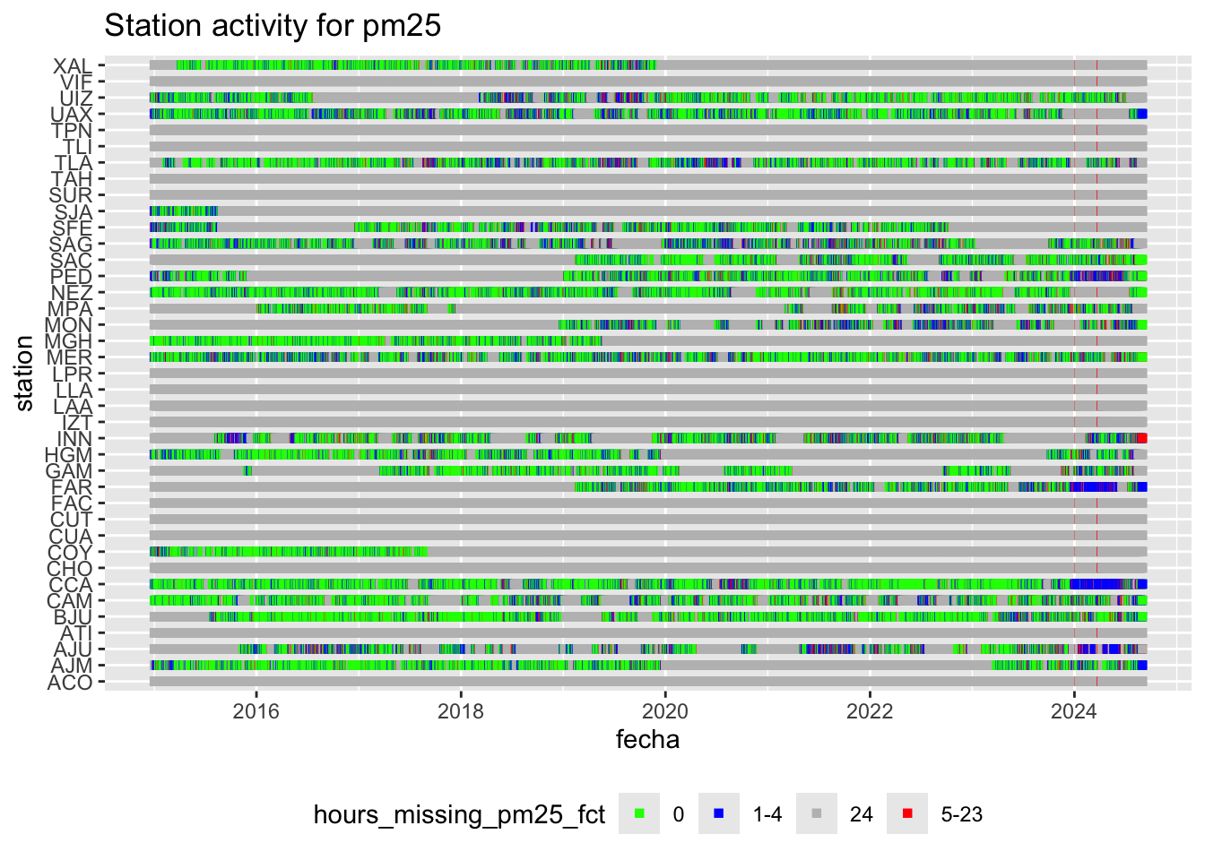
ggsave(here("..", "output",
            "figures",
            "stations_activity_pollution.png"),
       width = 10,
       height = 10,
       dpi = 300)
Matching procedure
Now, I want to go from station level to AGEB level. This is quite heavy because I want to work at the hourly level.
I compute a distance weighted average of all variables for eahc AGEB and each hour of each day. I then compute daily averages for every AGEB.
I have 3143 days and 24 hourly measures for each. I have to do it day by day, to not exhaust memory. I assign to each AGEB per day per hour the measures of all stations within 20km. I then compute a distance weighted avergae for each hour. Finally, I compute daily averages to end up at the day per AGEB level.
# this long function computes daily averages at the AGEB level
# from hourly data at the station level
# It also takes care of missing values

process_data_for_one_day <- function(fecha) {

  hourly_data_one_day <- hourly_data %>%
    filter(fecha == !!fecha)

  one_day_hourly <-
    # take each AGEB and station combination that are within 20km of each other
    distances %>% select(ageb, station, distance) %>%
    # add date to each observation
    mutate(fecha = hourly_data_one_day %>% pull(fecha) %>% unique(), .before = 1) %>%
    # multiply each obs by number of hours
    expand_grid(hora = 1:24) %>% relocate(hora, .after = "fecha") %>%
    # Add the actual data (day x station x hour) to each AGEB
    left_join(hourly_data_one_day,
              by = c("station", "fecha", "hora")) %>%
    # Now, i want to move to the AGEB by date by hour level
    # I take inverse distance weighted averages, so I compute a weight based on distance
    mutate(weight = 1/distance) %>%
    group_by(ageb, fecha, hora) %>%
    # compute idw averages
    summarise(across(.cols = co:so2,
                     .fns = ~ weighted.mean(., weight, na.rm = T)),
              .groups = "drop")

  one_day <- one_day_hourly %>%
    # Summarise hourly data to daily observations
    #I reduce each day to a single observation, by applying different functions.
    group_by(ageb, fecha) %>%
    summarise(
      #i want to count number of missing hours per day x AGEB
      across(co:so2, ~ sum(is.na(.)), .names = "nr_hrs_NA_{.col}"),
      # If all hours are recorded, i take mean max min...
      # if 1-4 are missing, i still take an average, max, min
      # if more than 4 hours are missing (or all), I want to set the value to NA
      pm25_hourly = list(pm25),
      pm10_hourly = list(pm10),

      co =
        if_else(nr_hrs_NA_co > 4, NA, mean(co, na.rm = T)),
      no =
        if_else(nr_hrs_NA_no > 4, NA, mean(no, na.rm = T)),
      no2 =
        if_else(nr_hrs_NA_no2 > 4, NA, mean(no2, na.rm = T)),
      nox =
        if_else(nr_hrs_NA_nox > 4, NA, mean(nox, na.rm = T)),
      o3 =
        if_else(nr_hrs_NA_o3 > 4, NA, mean(o3, na.rm = T)),
      pmco =
        if_else(nr_hrs_NA_pmco > 4, NA, mean(pmco, na.rm = T)),
      so2 =
        if_else(nr_hrs_NA_so2 > 4, NA, mean(so2, na.rm = T)),

      .groups = "drop"
    ) %>%
    select(-nr_hrs_NA_co, -nr_hrs_NA_no, -nr_hrs_NA_no2, -nr_hrs_NA_nox,
           -nr_hrs_NA_o3, -nr_hrs_NA_pmco, -nr_hrs_NA_so2)

  return(one_day)
}

# just as an example for one day.
# I have one observation per AGEB.
# process_data_for_one_day(fechas[1])
# process_data_for_one_day(fechas[3])
Run the procedure on each day, bind and save data
# To test the code on a small subset
# hourly_data <- hourly_data %>%
#    filter(fecha %in% seq(as.Date("2019-01-01"), as.Date("2019-01-31"), "days"))

# get all the different dates
fechas <- hourly_data %>%
  pull(fecha) %>%
  unique()

# set parallel computing
parallel::detectCores()
[1] 10plan(multisession, workers = 6)
# set memory limit
mem.maxVSize(vsize = 40000)[1] 40000# run for each day
tic()
list_of_days <-
# use map insetad of future_map to run single core with purrr
future_map(fechas, ~ process_data_for_one_day(.x),
.progress = TRUE)
toc() 7438.517 sec elapsed# to go back to single core
plan(sequential)
#Bind the dataframes
pollution_daily <-
list_rbind(list_of_days)
# Save the data
pollution_daily %>%
write_rds(here("..", "output",
"temporary_data",
"weather",
"processed_rama_20_ageb.rds"),
compress = "gz")