all_files <-
  # get full path
  tibble(path = list.files(here("..", "raw_data", "3_aire_cdmx", "EXCEL_new"),
                           # careful, 2023WSP.xlsx for some reason!!
                           pattern = ".*xls",
                           recursive = T,
                           full.names = T))

all_files <- all_files %>%
  mutate(basename = basename(path),
         basename = str_remove(basename, ".xlsx"),
         basename = str_remove(basename, ".xls"),
         year_file = as.numeric(str_sub(basename, 1, 4)),
         variable = str_sub(basename, 5),
         source = str_extract(path, "(?<=EXCEL_new/)[^/]+")) %>%
  filter(source == "REDMET") %>%
relocate(path, .after = everything())Weather data from REDMET
Note
In this script, I wrangle the weather data. I downloaded it from aire.cdmx.gob.mx in EXCEL format. Then they sent me the updates via email, because the site went down. The source that measures at the station by hour level for Mexico City. - REDMET (Red de Meteorología y Radiación Solar) for temperature, humidity, wind speed and wind direction
Warning
Warning: Script takes hours to run on my computer (or 30mins with parallelization x6)
Some parameters: - I remove a measured day if more than 4 hours out of 24 are missing - Inverse distance weight within 20km
Import REDMET hourly data
First, list all the excel files.
Import all the data and join into a single dataframe.
# import all the data in lists
hourly_data <-
  map(all_files %>% pull(variable) %>% unique(), ~{
    print(paste0("Importing: ", .x))

    all_files %>%
      filter(variable == .x) %>%
      pull(path) %>%
      map(~ read_excel(.)) %>%
      list_rbind() %>%
      pivot_longer(cols = -c(FECHA, HORA),
                   names_to = "station",
                   values_to = .x)
  }, .progress = TRUE)
[1] "Importing: PA"
[1] "Importing: RH"
[1] "Importing: TMP"[1] "Importing: WDR"
[1] "Importing: WSP"#reduce the lists by dataset
hourly_data <- hourly_data %>%
reduce(full_join, by = c("FECHA", "HORA", "station"))
#rename and encode
hourly_data <- hourly_data %>%
rename_with(tolower) %>%
mutate(fecha = as_date(fecha))
rm(all_files)Look at missing data in the weather data
# encode missing variables!
hourly_data <- hourly_data %>%
  mutate(across(where(is.numeric), ~ na_if(., -99)))

# make complete to be able to understand how much is missing
hourly_data <- hourly_data %>%
  complete(station, fecha, hora)

# remove pressure, its always missing
hourly_data <- hourly_data %>%
  select(-pa)

# We dont care about 2015
hourly_data <- hourly_data %>%
  filter(year(fecha) %in% 2016:2025)
Most of the 30 stations have at some point some data for some variables.
missing_summary <- hourly_data %>%
  group_by(station, year = year(fecha)) %>%
  summarise(across(.cols = where(is.numeric) & !hora,
                   .fns = ~ sum(is.na(.)) / n())) %>%
  pivot_longer(cols = -c(station, year), names_to = "variable", values_to = "missing_pct")

missing_summary %>%
  group_by(station, variable) %>%
  summarise(missing_pct = mean(missing_pct)) %>%
  ggplot(aes(x = variable, y = station, fill = missing_pct)) +
  geom_tile(color = "white", size = 1) +
  scale_fill_gradient(low = "green", high = "red", name = "Missing %") +
  geom_text(aes(label = scales::percent(missing_pct, accuracy = 1)),  # Format as % with 1 decimal
            color = "black", size = 3) +  # Adjust size and color of text
  theme_light() +
  theme(axis.text.x = element_text(angle = 45, hjust = 1))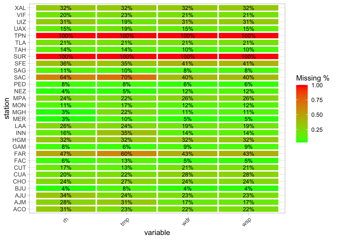
missing_summary %>%
  ggplot(aes(x = variable, y = station, fill = missing_pct)) +
  geom_tile(color = "white", size = 1) +
  scale_fill_gradient(low = "green", high = "red", name = "Missing %") +
  theme_light() +
  theme(axis.text.x = element_text(angle = 45, hjust = 1)) +
  scale_y_discrete(guide = guide_axis(n.dodge = 2)) +
  facet_wrap(~year)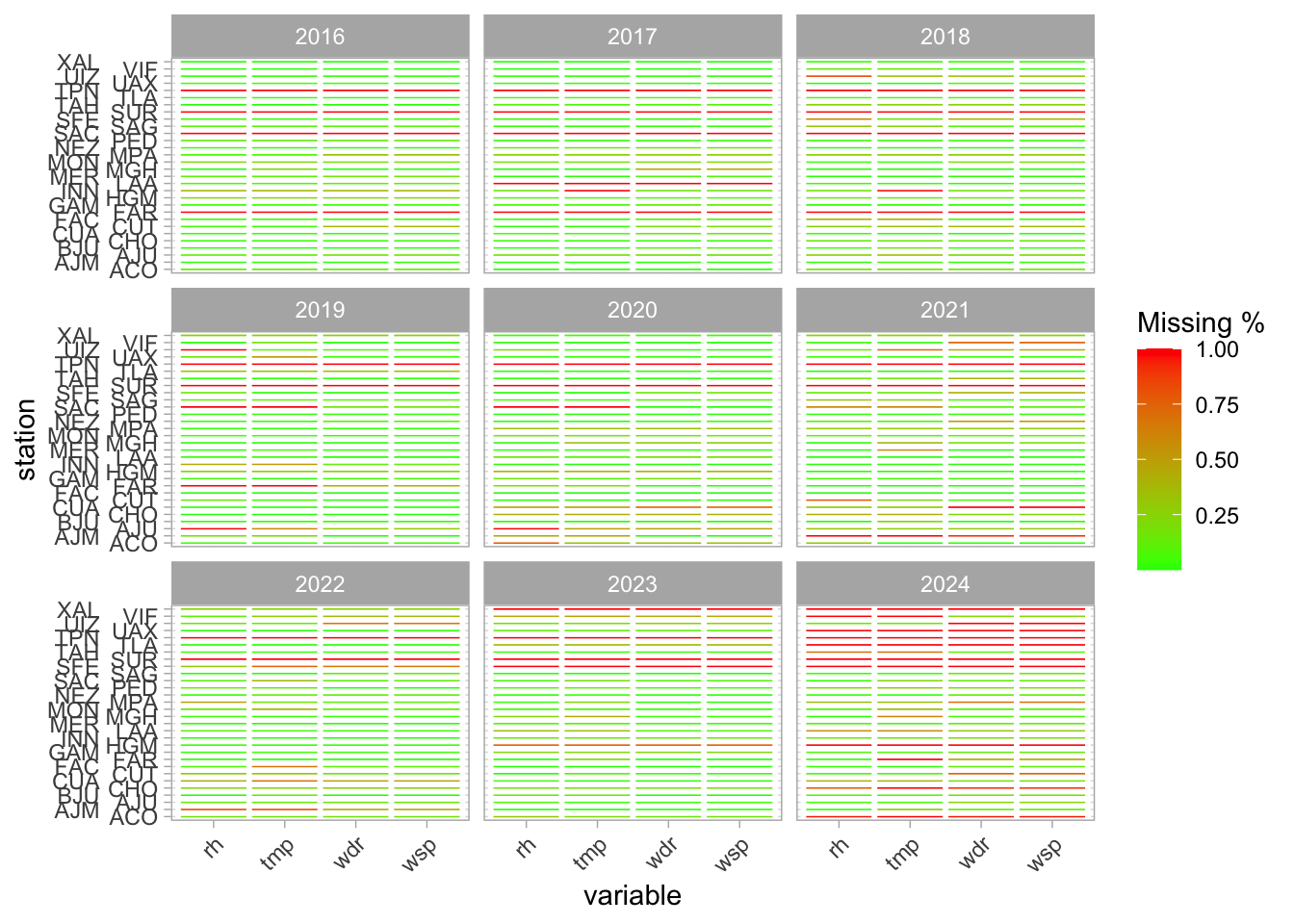
Still, I remove SUR and TPN. FAR and SAC turn on at some point, so I keep them. 2024 has little data……
hourly_data <- hourly_data %>%
  filter(!station %in% c("SUR", "TPN"))
We are going to look at daily averages. When doing so, it is crucial to know how many hours are missing for each day. For all variables, all 24 hours are recorded in 70% of the cases. Then, about 4% of the time, the station has some hours missing in the day. in 26% of the cases, all hours are NAs.
hourly_missings <- hourly_data %>%
  group_by(fecha, station) %>%
  summarise(across(rh:wsp, ~ sum(is.na(.)), .names = "hours_missing_{.col}")) %>%
  mutate(across(starts_with("hours_missing"), ~ case_when(. == 0 ~ "0",
                                                          . == 1 ~ "1",
                                                          . %in% 2:23 ~ "2-23",
                                                          . == 24 ~ "24"),
                .names = "{.col}_fct")) %>% ungroup()

hourly_missings %>% count(hours_missing_tmp) %>% mutate(prop = n / sum(n)) %>% kable()| hours_missing_tmp | n | prop |
|---|---|---|
| 0 | 65420 | 0.7379749 |
| 1 | 2051 | 0.0231364 |
| 2 | 601 | 0.0067796 |
| 3 | 278 | 0.0031360 |
| 4 | 220 | 0.0024817 |
| 5 | 144 | 0.0016244 |
| 6 | 114 | 0.0012860 |
| 7 | 118 | 0.0013311 |
| 8 | 91 | 0.0010265 |
| 9 | 76 | 0.0008573 |
| 10 | 68 | 0.0007671 |
| 11 | 67 | 0.0007558 |
| 12 | 73 | 0.0008235 |
| 13 | 81 | 0.0009137 |
| 14 | 106 | 0.0011957 |
| 15 | 62 | 0.0006994 |
| 16 | 33 | 0.0003723 |
| 17 | 20 | 0.0002256 |
| 18 | 18 | 0.0002031 |
| 19 | 10 | 0.0001128 |
| 20 | 8 | 0.0000902 |
| 21 | 7 | 0.0000790 |
| 22 | 8 | 0.0000902 |
| 23 | 23 | 0.0002595 |
| 24 | 18951 | 0.2137781 |
hourly_missings %>% count(hours_missing_tmp_fct) %>% mutate(prop = n / sum(n)) %>% kable()| hours_missing_tmp_fct | n | prop |
|---|---|---|
| 0 | 65420 | 0.7379749 |
| 1 | 2051 | 0.0231364 |
| 2-23 | 2226 | 0.0251105 |
| 24 | 18951 | 0.2137781 |
We can plot this station recording activity for temperatture over time:
hourly_missings %>%
  ggplot(aes(x = fecha, y = station, col = hours_missing_tmp_fct)) +
  geom_point(shape = 15) +
  scale_color_manual(values = c("0" = "green", "1" = "blue",
                                "2-23" = "red", "24" = "gray")) +
  labs(title = "Station activity for temperature") +
  theme(legend.position = "bottom")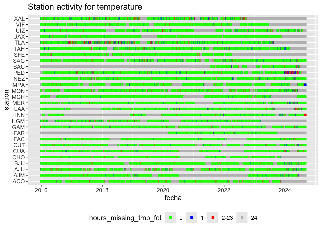
ggsave(here("..", "output",
            "figures",
            "stations_activity_weather.png"),
       width = 10,
       height = 10,
       dpi = 300)
I want to plot the distribution of raw temperatures, just a quick sanity check.
hourly_data %>%
  ggplot(aes(x = tmp)) +
  geom_density() +
  labs(title = "Distribution of raw temperatures",
       x = "Temperature (°C)",
       y = "Frequency")
hourly_data %>%
  mutate(tmp_rounded = round(tmp, 0)) %>%
  count(tmp_rounded) %>%
  mutate(freq = n / sum(n)) %>%
  ggplot(aes(x = tmp_rounded, y = freq)) +
  geom_bar(stat = "identity") +
  scale_y_continuous(labels = scales::percent_format()) +
  labs(title = "Distribution of raw temperatures",
       x = "Temperature (°C)",
       y = "Frequency")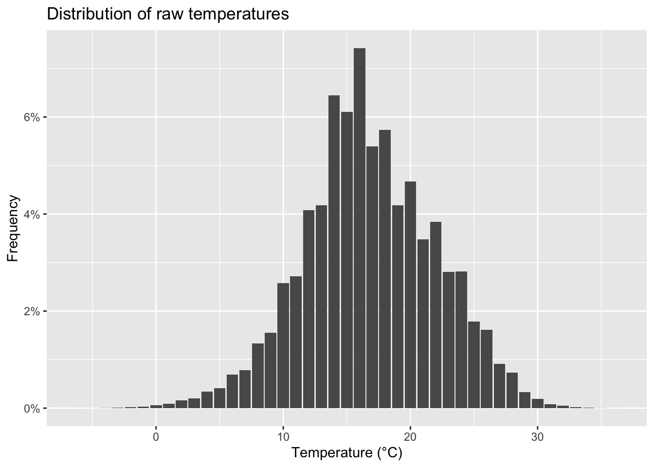
Now, move to the AGEB level
This is quite heavy because I want to work at the hourly level. I compute a distance weighted average of all variables for each AGEB and each hour of each day. I then compute daily averages for every AGEB.
Distances between stations and AGEBs
Location of all the stations
catalogo_est <-
  read_csv(here("..",
                "raw_data",
                "3_aire_cdmx",
                "cat_estacion.csv"),
           skip = 1,
           locale = readr::locale(encoding = "latin1")) %>%
  rename(station = cve_estac)

# all the stations are in the catalog
catalogo_est <- catalogo_est %>%
  filter(station %in% (hourly_data %>% pull(station) %>% unique()))
Locations of the AGEB, and their centroids.
catalogo_ageb <-
  read_sf(here("..",
                "output",
                "ageb_poligonos.geojson"),
          quiet = TRUE) %>%
  st_transform(4326)

catalogo_ageb <- catalogo_ageb %>%
  st_centroid() %>%
  mutate(lon = st_coordinates(.)[, 1],
         lat = st_coordinates(.)[, 2]) %>%
  st_drop_geometry() %>% as_tibble()
I want to compute the distances between each station and the centroid of each AGEB.
# Compute the distances between each station and the col centroids
# create a df from all combinations of stations and municipalities
distances <-
  crossing(
    (catalogo_ageb %>% select(ageb,
                             ageb_lon = lon,
                             ageb_lat = lat)),
    (catalogo_est %>% select(station,
                             sta_lon = longitud,
                             sta_lat = latitud))
  )

# compute the distance in meters, using haversine method, and convert to km
distances <- distances %>%
  mutate(distance = geosphere::distHaversine(cbind(ageb_lon, ageb_lat),
                                             cbind(sta_lon, sta_lat)),
         distance = distance/1000)

distances %>%
  write_rds(here("..", "output",
                 "temporary_data",
                 "weather",
                 "distances_weather.rds"))

#Only keep the combinations that are within 20km
distances <- distances %>%
  filter(distance <= 20)
Matching procedure
I have 3143 days and 24 hourly measures for each. I have to do it day by day, to not exhaust memory. I assign to each AGEB per day per hour the measures of all stations within 20km. I then compute a distance weighted avergae for each hour. Finally, I compute daily averages to end up at the day per AGEB level.
# this long function computes daily averages at the AGEB level
# from hourly data at the station level
# It also takes care of missing values

process_data_for_one_day <- function(fecha) {

  hourly_data_one_day <- hourly_data %>%
    filter(fecha == !!fecha)

  one_day_hourly <-
    # take each AGEB and station combination that are within the cutoff distance of each other
    distances %>% select(ageb, station, distance) %>%
    # add date to each observation
    mutate(fecha = hourly_data_one_day %>% pull(fecha) %>% unique(), .before = 1) %>%
    # multiply each obs by number of hours
    expand_grid(hora = 1:24) %>% relocate(hora, .after = "fecha") %>%
    # Add the actual data (day x station x hour) to each AGEB
    left_join(hourly_data,
              by = c("station", "fecha", "hora")) %>%
    # Now, i want to move to the AGEB by date by hour level
    # I take inverse distance weighted averages, so I compute a weight based on distance
    mutate(weight = 1/distance) %>%
    group_by(ageb, fecha, hora) %>%
    # compute idw averages
    summarise(across(.cols = rh:wsp,
                     .fns = ~ weighted.mean(., weight, na.rm = T)),
              .groups = "drop")

  one_day <- one_day_hourly %>%
    # Summarise hourly data to daily observations
    #I reduce each day to a single observation, by applying different functions.
    group_by(ageb, fecha) %>%
    summarise(
      #i want to count number of missing hours per day x AGEB
      across(rh:wsp, ~ sum(is.na(.)), .names = "nr_hrs_NA_{.col}"),
      # If all hours are recorded, i take mean max min...
      # if only one hour is missing, i still take an average, max, min
      # if more than one (or all) hours are missing, I want to set the value to NA

      rh =
        if_else(nr_hrs_NA_rh > 1, NA, mean(rh, na.rm = T)),
      wdr =
        if_else(nr_hrs_NA_wdr > 1, NA, mean(wdr, na.rm = T)),
      wsp =
        if_else(nr_hrs_NA_wsp > 1, NA, mean(wsp, na.rm = T)),

      tmp_hourly = list(tmp),

      .groups = "drop"
    ) %>%
    select(-nr_hrs_NA_rh, -nr_hrs_NA_wdr, -nr_hrs_NA_wsp)

  return(one_day)
}
Run the procedure on each day, bind and save data
# for testing, select just a few days
# hourly_data <- hourly_data %>%
#    filter(fecha %in% seq(as.Date("2019-01-01"), as.Date("2019-01-31"), "days"))

# get all the different dates
fechas <- hourly_data %>%
  pull(fecha) %>%
  unique()

# set parallel computing
parallel::detectCores()
[1] 10plan(multisession, workers = 6)
# set memory limit
mem.maxVSize(vsize = 40000)[1] 40000# run for each day
tic()
list_of_days <-
# use map insetad of future_map to run single core with purrr
future_map(fechas, ~ process_data_for_one_day(.x),
.progress = TRUE)
toc() 2836.872 sec elapsed# to go back to single core
plan(sequential)
#Bind the dataframes
weather_daily <-
list_rbind(list_of_days)
# Save the data
weather_daily %>%
write_rds(here("..", "output",
"temporary_data",
"weather",
"processed_redmet_20_ageb.rds"),
compress = "gz")