Crime data from Attorney General’s Office

Note

In this script, I import the raw crime data. I clean the data, and compute the delay in reporting. I look at crime types and categorise them in broader categories. I then assign AGEBs to each crime based on the coordinates.

I save the cleaned crime level data in PGJ_carpetas.rds and plot some trends.

The crime data come from from Mexico City Attorney General’s Office (FGJCDMX in its Spanish initials, https://www.fgjcdmx.gob.mx/). The data consist of administrative incident report records starting in 2016 to today for incidents happening in Mexico City. Each entry contains information on the type of crime, date, time and precise geographic coordinates of the incident. Crime include domestic violence, homicides, various types of robbery and larceny… I select domestic violence crime.

1 Import the incident level data

carpetas <-
  fread(here("..",
             "raw_data",
             "5_pgj_cdmx",
             "carpetas_de_investigacion",
             "carpetasFGJ_acumulado_2024_09.csv.zip"),
        colClasses = 'character')

These data contain four types of info:

1. Date and time of incident
2. Type of incident
3. Police department that investigated the case
4. Precise location of the incident

Create a unique ID for each crime report:

carpetas <-  carpetas %>% 
  mutate(c_id = row_number(), .before = 1) %>% 
  as_tibble()

2 Dates and time

Clean the dates variables

There are 4 variables for each of two dates: - Date on which the incident was opened by the police - Date of the incident (which is much more important for my analysis).

I keep both:

carpetas <- carpetas %>% 
  filter(!is.na(fecha_hecho)) %>% 
  mutate(date = ymd(fecha_hecho),
         dttm = ymd_hms(paste(fecha_hecho, hora_hecho)),
         .after = 1)

carpetas <- carpetas %>% 
  select(-anio_inicio, -mes_inicio,
         -anio_hecho, -mes_hecho, -fecha_hecho, -hora_hecho)

Filter incidents based on dates

The data covers all cases opened in 2016 upwards. However, they can concern incident that happened before. I select incidents which happened between 2016 and 2024. A case that happened in 2015 could be in the data, but could also not, depending on when the case has been opened, so I exclude older years.

carpetas <- carpetas %>% 
  filter(year(date) %in% 2016:2024)

# exclude the last month of data, incomplete
carpetas <- carpetas %>% 
  filter(!(year(date) == year(max(carpetas$date)) &
             month(date) == month(max(carpetas$date))))

Here is the daily count of all the incidents in our data.

carpetas %>% group_by(date = date) %>%
  count(. , sort = TRUE) %>% 
  ggplot(., aes(x=date, y=n)) +
  geom_line() +
  xlab("") +
  ylab("Number of daily cases")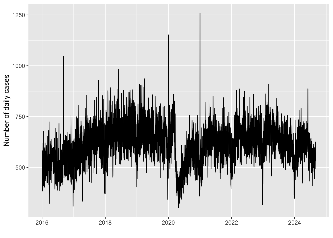

The most striking feature of this figure is that the lockdown generated a large decrease in incident reports.

3 Compute the time delay in reporting

We have two dates: - occurrence time, according to the victim (fecha y hora en que se cometió el delito, según el reporte de la víctima.) - date and time of complaint (fecha y hora en que se hizo la denuncia para iniciar la carpeta de investigación.)

First, look at the missing values for the hours. We have all hours recorded for hecho, but 75% of 00:00:00 in the inicio time (time the case was opened). This is because they only started recording the hour from 2022-07-01 onwards. I encode all these 00:00:00 in hora_inicio as NAs.

carpetas %>% 
  mutate(hora_hecho = hms::as_hms(dttm)) %>% 
  ggplot(aes(hora_hecho)) +
  geom_density() +
  labs(title = "no missing hours in the hecho time")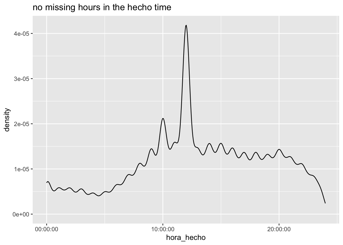

#but 75% of 00:00:00 in the inicio time
carpetas %>% 
  count(hora_inicio, sort = T) %>% 
  mutate(freq = n/sum(n)) %>% 
  head(3) %>% kable()

hora_inicio	n	freq
00:00:00	1454167	0.7347632
13:16:00	185	0.0000935
13:24:00	185	0.0000935

# this is because they only started recording the hour from 2022-07-01
carpetas %>% 
  group_by(year = year(ymd(fecha_inicio))) %>%
  summarise(share_of_000000 = mean(hora_inicio == "00:00:00", na.rm = T)) %>% 
  kable()

year	share_of_000000
2016	1.0000000
2017	1.0000000
2018	1.0000000
2019	1.0000000
2020	1.0000000
2021	0.9999869
2022	0.4920488
2023	0.0000207
2024	0.0003999
NA	NaN

#everything is 00:00:00 before, and only very few after, so i assume those 00 are actually midnight
carpetas %>% 
  group_by(before = ymd(fecha_inicio) < ymd("2022-07-01")) %>% 
  summarise(share_of_000000 = mean(hora_inicio == "00:00:00", na.rm = T)) %>% 
  kable()

before	share_of_000000
FALSE	0.0001371
TRUE	0.9999931
NA	NaN

# so i mark them as NA
carpetas <- carpetas %>% 
  mutate(hora_inicio =
           if_else(ymd(fecha_inicio) < ymd("2022-07-01"),NA, hora_inicio),
         fecha_inicio = ymd(fecha_inicio))

Now i can actually compute the delay in reporting.

Delay in day for full sample

I can compute the delay in days for the whole sample.

carpetas <- carpetas %>% 
  mutate(delay_full_days =
           as.numeric(difftime(fecha_inicio, date, units = "days")))

#remove a few negative delays and 2 NA
carpetas %>% 
  count(delay_full_days >= 0)

# A tibble: 3 × 2
  `delay_full_days >= 0`       n
  <lgl>                    <int>
1 FALSE                      110
2 TRUE                   1978983
3 NA                           3

carpetas <- carpetas %>% 
  filter(delay_full_days >= 0)

Look at deciles and plot distribution of delays in full days.

#compute decile
carpetas <- carpetas %>% 
  mutate(decile_delay_full_days = ntile(delay_full_days, 10))
  
#show decile stats
carpetas %>% 
  group_by(decile_delay_full_days) %>%
  summarize(min(delay_full_days),
            max(delay_full_days),
            n = n())

# A tibble: 10 × 4
   decile_delay_full_days `min(delay_full_days)` `max(delay_full_days)`      n
                    <int>                  <dbl>                  <dbl>  <int>
 1                      1                      0                      0 197899
 2                      2                      0                      0 197899
 3                      3                      0                      0 197899
 4                      4                      0                      1 197898
 5                      5                      1                      1 197898
 6                      6                      1                      2 197898
 7                      7                      2                      5 197898
 8                      8                      5                     15 197898
 9                      9                     15                     57 197898
10                     10                     57                   3144 197898

# plot distribution of delays
carpetas %>% 
  filter(decile_delay_full_days <= 9) %>% 
  ggplot(aes(delay_full_days)) +
  geom_histogram(binwidth = 1, aes(y = after_stat(count) / sum(after_stat(count)))) +
  labs(title = "Distribution of days of delay in reporting (exluding top 10%)",
       x = "Delay in days",
       y = "Share") +
    scale_y_continuous(labels = scales::percent_format())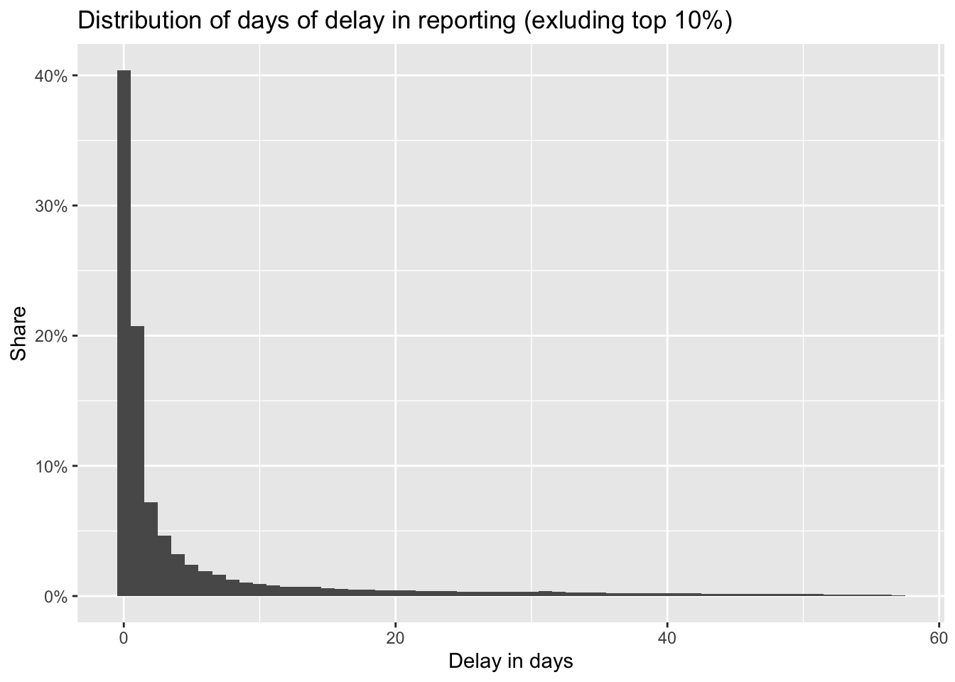 

Delay in hours for the recent data

For the delay in continuous time (as opposed to full days), I only have enough information for second half of 2022 onwards.

carpetas <- carpetas %>% 
  mutate(dttm_inicio = ymd_hms(paste0(fecha_inicio, hora_inicio)))

carpetas <- carpetas %>% 
  mutate(delay_hours = as.numeric(dttm_inicio - dttm)/3600)

#encode negative delays
carpetas %>% 
  count(delay_hours >= 0)

# A tibble: 3 × 2
  `delay_hours >= 0`       n
  <lgl>                <int>
1 FALSE                 3915
2 TRUE                520725
3 NA                 1454343

carpetas <- carpetas %>% 
  filter(delay_hours >= 0 | is.na(delay_hours))

Look at decile and plot distribution

carpetas <- carpetas %>% 
  mutate(decile_delay_hours = ntile(delay_hours, 10))

carpetas %>% 
  group_by(decile_delay_hours) %>%
  summarize(min(delay_hours),
            max(delay_hours),
            n = n())

# A tibble: 11 × 4
   decile_delay_hours `min(delay_hours)` `max(delay_hours)`       n
                <int>              <dbl>              <dbl>   <int>
 1                  1               0                  1.57   52073
 2                  2               1.57               4.28   52073
 3                  3               4.28              10.0    52073
 4                  4              10.0               22.1    52073
 5                  5              22.1               40.5    52073
 6                  6              40.5               75.8    52072
 7                  7              75.8              168.     52072
 8                  8             168.               489.     52072
 9                  9             489.              1874.     52072
10                 10            1874.             75450.     52072
11                 NA              NA                 NA    1454343

carpetas %>% 
  select(delay_hours) %>% arrange(delay_hours) %>% 
  mutate(round_delay_hours = round(delay_hours, 0)) %>%
  count(round_delay_hours) %>% 
  mutate(share = n/sum(n)) %>% 
  ggplot(aes(round_delay_hours, share)) +
  geom_bar(stat = "identity") +
  labs(title = "Distribution of hours of delay in reporting (zooming on 0-72 hours)",
       x = "Delay in hours",
       y = "Share") +
  scale_x_continuous(breaks = seq(0, 72, 12)) +
  scale_y_continuous(labels = scales::percent_format()) +
  coord_cartesian(xlim = c(0, 72))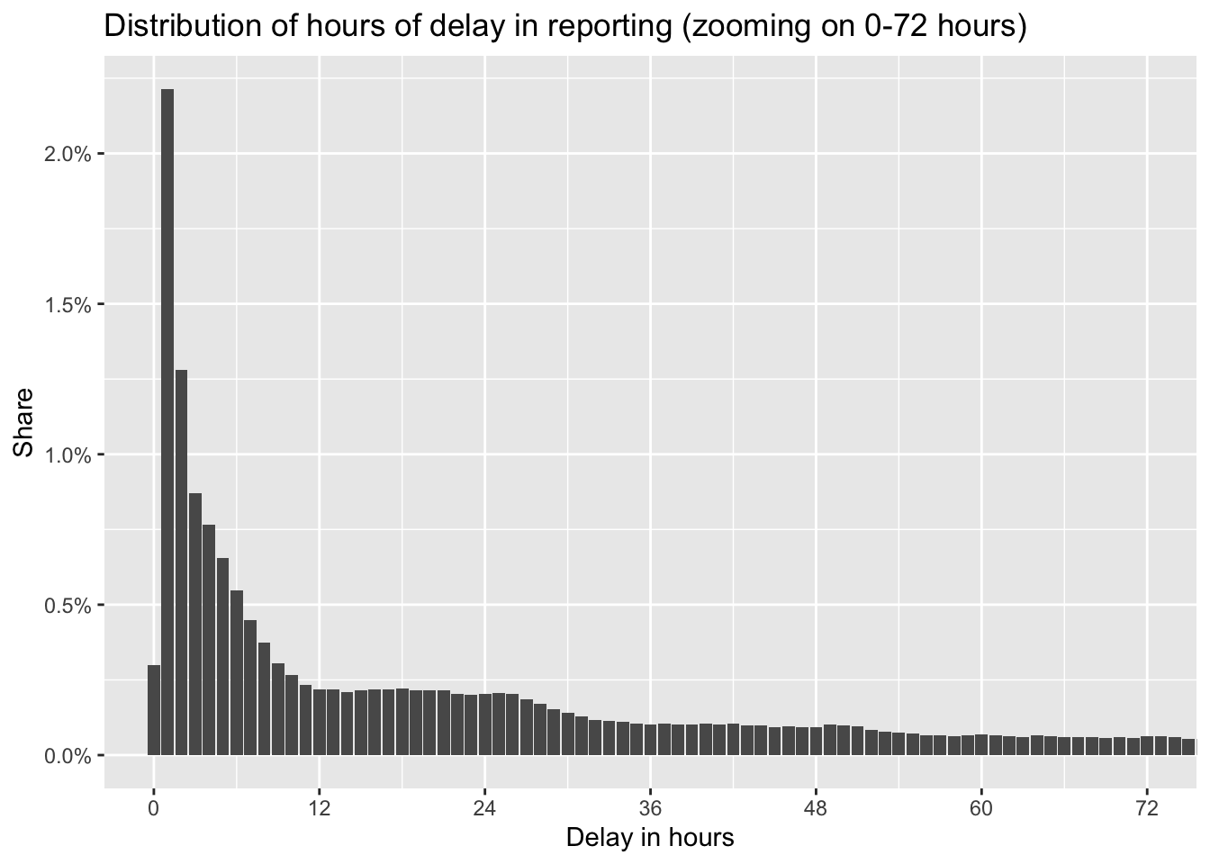

4 Type of crimes

There are two variables to understand what the crime is delito and categoria_delito.

categoria_delito contains only 18 broad categories, and the vast majority is classified as “low impact crime”. This is not useful to classify crimes.

carpetas %>%
  count(categoria_delito, sort = TRUE) %>% 
  ggplot(aes(categoria_delito, n)) +
  geom_col() +
  coord_flip() +
  ylab("categoria_delito")

carpetas <- carpetas %>% 
  select(-categoria_delito)
# all DV crimes are qualified as "delito the bajo impacto" anyways

The second variable, delito, allows to identify the nature of crimes. Es la conducta, acción u omisión típica (descrita por la ley), antijurídica (contraria a la ley) y culpable, a la que le corresponde una sanción.

# First, explore the kind of delitos, just to have an idea
carpetas %>% count(delito, sort=T) %>%
  mutate(prop = round(100*n/sum(n), 2)) %>% 
  arrange(desc(n)) %>% 
  head(8) %>% kable()

delito	n	prop
VIOLENCIA FAMILIAR	245061	12.41
FRAUDE	140654	7.12
AMENAZAS	127593	6.46
ROBO DE OBJETOS	108253	5.48
ROBO A TRANSEUNTE EN VIA PUBLICA CON VIOLENCIA	85545	4.33
ROBO A NEGOCIO SIN VIOLENCIA	74710	3.78
ROBO DE ACCESORIOS DE AUTO	70127	3.55
ROBO DE OBJETOS DEL INTERIOR DE UN VEHICULO	55098	2.79

carpetas %>% distinct(delito) %>% nrow()

[1] 352

There are 350+ types of delitos. These are the most common.

carpetas %>% 
  mutate(delito = fct_infreq(delito)) %>%
  mutate(delito = fct_lump_n(delito, n = 10)) %>% 
  ggplot(aes(delito)) +
  geom_bar() +
  coord_flip()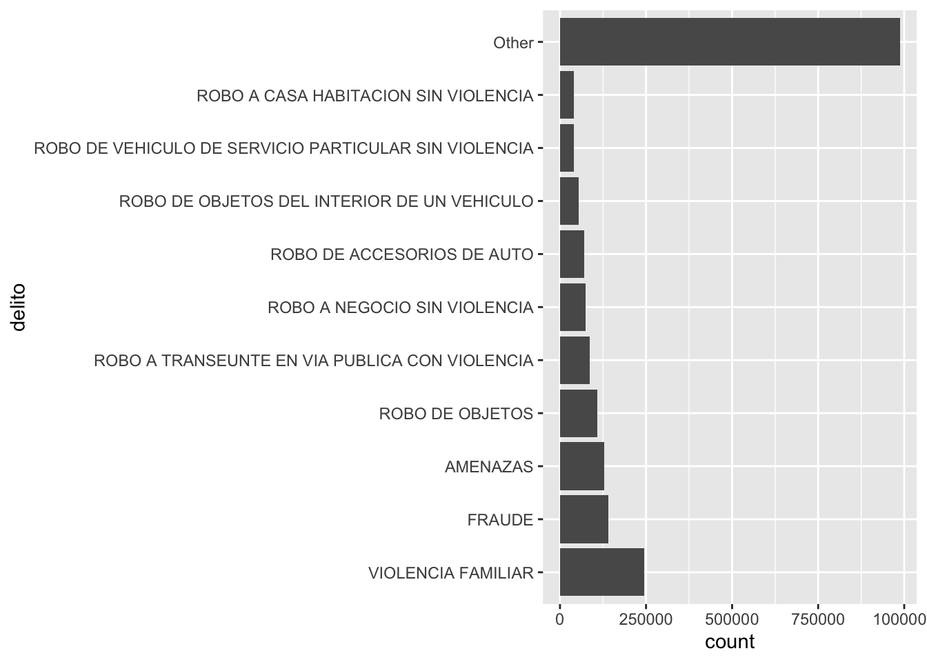

There is a lot of categories that could be lumped together. There are e.g. 120 subtypes of theft, which I want to group into a category. So I create new broader categories, with the most frequent/relevant types of crime.

carpetas <- carpetas %>% 
  mutate(delito_lumped = case_when(
    delito == "VIOLENCIA FAMILIAR"      ~ "Domestic violence",
    delito == "FRAUDE"                  ~ "Fraud",
    delito == "AMENAZAS"                ~ "Threats",
    delito == "ABUSO DE CONFIANZA"      ~ "Trust abuse",
    str_detect(delito, "ROBO")          ~ "Theft",
    str_detect(delito, "SEXUAL")        ~ "Sexual crimes",
    str_detect(delito, "VIOLACION")     ~ "Rapes",
    str_detect(delito, "SUICIDIO")      ~ "Suicides",
    str_detect(delito, "NARCO")         ~ "Drugs related",
    str_detect(delito, "HOMICIDIO")     ~ "Homicide",
    str_detect(delito, "FEMINICIDIO")   ~ "Feminicide",
    TRUE                                ~ "Other"),
    .after = "delito")

Plot the frequency of the new broad categories of crime, also includes the subcategories. There is no sub category for DV.

categories <- carpetas %>%
  count(delito_lumped, delito) %>% 
  group_by(delito_lumped) %>% 
  add_tally(sum(n), name = "lumped_total") %>% 
  arrange(desc(lumped_total), desc(n)) %>% 
  relocate(delito, .after = lumped_total)

categories %>% 
  ggplot(aes(area = n, fill = delito_lumped,
             label = delito,
             subgroup = delito_lumped)) +
  geom_treemap() +
  theme(legend.position = "none") +
  geom_treemap_subgroup_border() +
  geom_treemap_subgroup_text(place = "topleft",
                             alpha = 0.5, colour ="black",
                             min.size = 0) +
  scale_fill_brewer(palette = "Set3")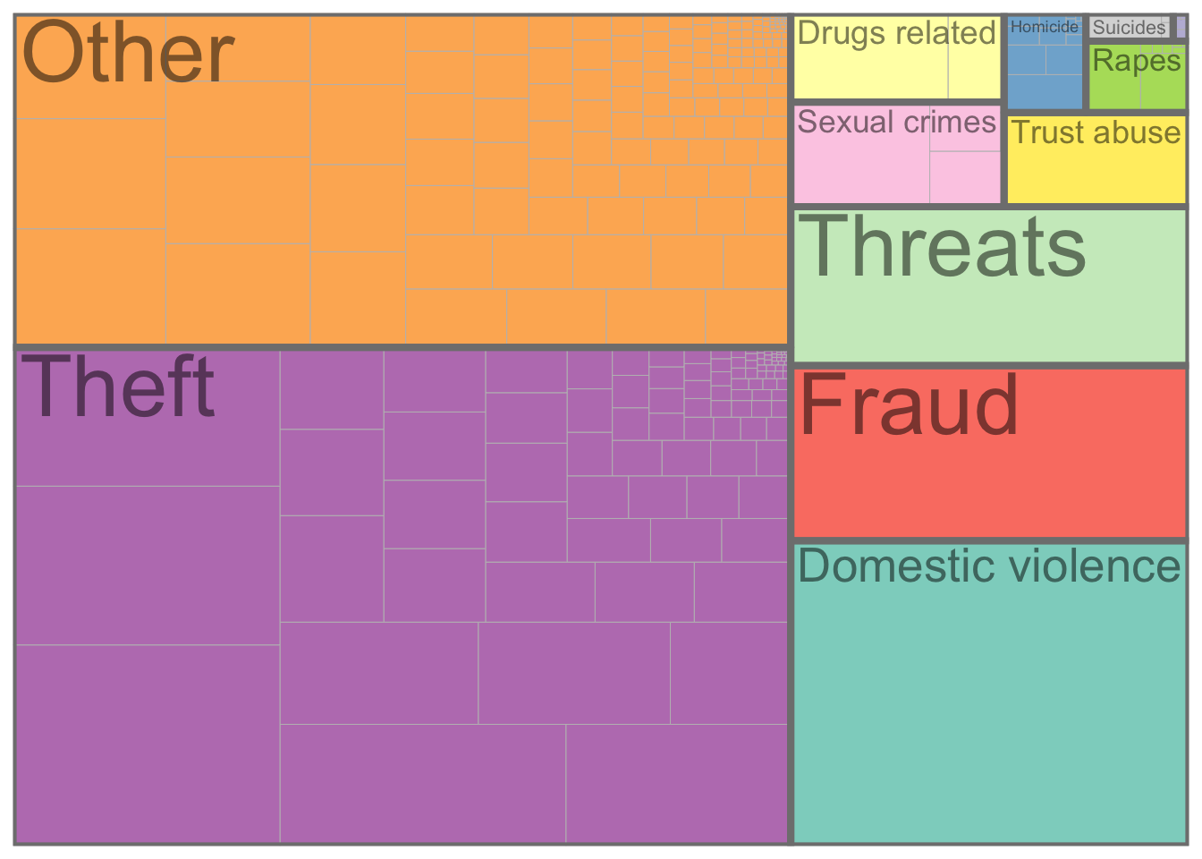

#  scale_fill_manual(values = colorRampPalette(brewer.pal(5, "PuOr"))(12))
# library(RColorBrewer)

categories <- categories %>% 
  filter(!delito_lumped %in% c("Theft"))

rm(categories)

5 Extra variables contained in the data

Mexico City Attorney General’s Office (https://www.fgjcdmx.gob.mx/secretaria/acerca-de) is organised in different prosecutors office. The variable fiscalia tells us which office was in charge of the case. Some offices are specialise in a type of crime, such as the Fiscalía de Investigación del Delito de Violencia Familiar https://www.fgjcdmx.gob.mx/secretaria/estructura/331. However, some fiscalia are only territorial, and do not provide information on what type of cases they focus on.

I combine all the territorial offices into one, since we already have information on the location of the crime, this is not very helpful.

names(carpetas)

 [1] "c_id"                   "date"                   "dttm"                  
 [4] "fecha_inicio"           "hora_inicio"            "delito"                
 [7] "delito_lumped"          "competencia"            "fiscalia"              
[10] "agencia"                "unidad_investigacion"   "colonia_hecho"         
[13] "colonia_catalogo"       "alcaldia_hecho"         "alcaldia_catalogo"     
[16] "municipio_hecho"        "latitud"                "longitud"              
[19] "delay_full_days"        "decile_delay_full_days" "dttm_inicio"           
[22] "delay_hours"            "decile_delay_hours"    

carpetas <- carpetas %>%
  mutate(fiscalia = if_else(str_detect(fiscalia,"FISCALÍA DE INVESTIGACIÓN TERRITORIAL"),
                            "FISCALÍA DE INVESTIGACIÓN TERRITORIAL",
                            fiscalia)) %>% 
  mutate(fiscalia = if_else(str_detect(fiscalia,"INVESTIGACIÓN EN "),
                            "FISCALÍA DE INVESTIGACIÓN TERRITORIAL",
                            fiscalia)) 
#INVESTIGACIÓN EN ALCADIA ... is for 2016, 2017, 2018, 2019
#FISCALÍA DE INVESTIGACIÓN TERRITORIAL EN ALCADIA ... is for 2020, 2021, 2022
#But they're the same thing. I merge them

There are a 65 different prosecutor’s office, but in 80% of the cases, the office is a territorial one. So this variable is not very useful.

carpetas %>% count(fiscalia) %>% as_tibble() %>%
  arrange(desc(n)) %>% mutate(freq = round(100*n/sum(n),2)) %>% 
  filter(freq>0.1) %>% 
  head(8) %>% kable()

fiscalia	n	freq
FISCALÍA DE INVESTIGACIÓN TERRITORIAL	1531865	77.56
AGENCIA DE DENUNCIA DIGITAL	140213	7.10
FISCALÍA DE INVESTIGACIÓN DEL DELITO DE VIOLENCIA FAMILIAR	46660	2.36
FISCALÍA DE INVESTIGACIÓN DE DELITOS SEXUALES	34485	1.75
INVESTIGACIÓN PARA LA ATENCIÓN DE NIÑOS, NIÑAS Y ADOLESCENTES	26406	1.34
FISCALÍA DE INVESTIGACIÓN DE DELITOS COMETIDOS EN AGRAVIO DE NIÑAS, NIÑOS Y ADOLESCENTES	25237	1.28
FISCALÍA PARA LA INVESTIGACIÓN DE LOS DELITOS COMETIDOS POR SERVIDORES PÚBLICOS	21543	1.09
JUZGADOS FAMILIARES	20980	1.06

There are Agencias de Investigación, or agencies, which is not very relevant. https://www.sinembargo.mx/10-12-2013/840532

carpetas %>% count(fiscalia, agencia, sort = TRUE) %>% 
    head(6) %>% kable()

fiscalia	agencia	n
AGENCIA DE DENUNCIA DIGITAL	CEN-1	71885
FISCALÍA DE INVESTIGACIÓN TERRITORIAL	CUH-2	54203
FISCALÍA DE INVESTIGACIÓN TERRITORIAL	IZP-6	51855
FISCALÍA DE INVESTIGACIÓN TERRITORIAL	IZP-8	40588
FISCALÍA DE INVESTIGACIÓN TERRITORIAL	IZP-9	40116
FISCALÍA DE INVESTIGACIÓN TERRITORIAL	IZP-4	39907

Finally, there is a variable called unidad_investigacion. Again, not very useful. The only potential interesting thing is that they differentiate between sin detenido and con detenido.

carpetas %>% count(unidad_investigacion, sort=T) %>% 
    head(6) %>% kable()

unidad_investigacion	n
UI-1SD	681677
UI-1CD	213477
UI-2SD	206749
UI-3CD	198288
UI-2CD	192555
UI-3SD	171895

Finally, Competencia is a categorical variable that classifies events according to their nature.

carpetas %>% count(competencia, sort=T) %>% 
     kable()

competencia	n
NA	1035822
FUERO COMUN	909833
HECHO NO DELICTIVO	18644
INCOMPETENCIA	10769

There is a lot of missing data, so probably not very helpful.

Fuero común son los delitos que ocurren y se denuncian dentro de la Ciudad de México Hechos no delictivos corresponde a aquellos que son denunciados a la PGJ pero no constituyen un delito en sí mismos como por ejemplo un suicidio. Incompetencias son aquellos hechos delictivos que suceden fuera de CDMX y son denunciados a la PGJ de la CDMX, por lo que no se deben tomar en cuenta como incidencia delictiva propia de la ciudad. There are none of these cases for domestic violence crimes.

Overall, these extra variables do not provide useful information. I thus remove them.

carpetas <- carpetas %>%
  select(-fiscalia, -agencia,
         -unidad_investigacion, -competencia)

6 Location information

Location data consist of 6 variables: - “alcaldia_hecho” and “municipio_hecho”, - “colonia_hecho” and “colonia_catalogo”, - “longitud” and “latitud”.

The first two are at the district level. Districts is for CDMX, municipio for the rest of the country. This data is from the police report.

Then, the next two variables record the colonia, or neighborhood of the crime. colonia_hecho is the colonia as registered in the incident report while colonia_catalogo is automatically generated to be the colonia where the incident happened, based on the coordinates. Basically, they contain the same information, but with different spelling and abbreviations.

Finally, “longitud” and “latitud” are the coordinates of the incident.

In my analysis, I am going to rely on coordinates and assign AGEBs manually, based on these coordinates. This is what they did to assign the neighborhoods anyways.

Filter missing location data

I first remove the incidents that do not have coordinates data. They represent less than 5pc of the data, and also include all the crime that happened outside of CDMX (e.g. in surrounding states).

carpetas <- carpetas %>% filter(!(longitud == "0" | latitud == "0"))

Locate the crime reports by AGEBs

Import the reference AGEBs of CDMX

SHP of reference for AGEBs. There are 1948 of them, and I have population for each.

ageb <-  
  st_read(here("..",
                "output",
                "ageb_poligonos.geojson")) %>% 
  st_transform(4326) %>% 
  st_make_valid()

Reading layer `ageb_poligonos' from data source 
  `/Users/martin/Documents/EUI/RESEARCH/violence and climate/heat and DV mexico/data and regressions/output/ageb_poligonos.geojson' 
  using driver `GeoJSON'
Simple feature collection with 2431 features and 2 fields
Geometry type: POLYGON
Dimension:     XY
Bounding box:  xmin: -99.34306 ymin: 19.12409 xmax: -98.94664 ymax: 19.59276
Geodetic CRS:  WGS 84

Convert carpetas to a spatial object

Convert the carpetas to a spatial object in order to be able to compare it to the map of colonias. In the crime data, longitud and latitud variables are in “Geodetic CRS: WGS 84” (from the data dictionary). This corresponds to EPSG:4326 (see https://r.geocompx.org/reproj-geo-data.html#crs-in-r).

carpetas <-
  st_as_sf(carpetas,
           coords = c("longitud", "latitud"),
           crs = "EPSG:4326", # this is what the data dictionary says
           remove = FALSE) 

I plot it to verify its good. The crime locations and the map of the AGEBs do overlap geographically. I plot for one day.

# only select a day to not overload the plot
carpetas %>%
  filter(date == ymd("2020-07-14")) %>% 
  ggplot() +
  geom_sf(aes(color = delito_lumped)) +
  geom_sf(data = ageb, fill = NA, linewidth = .1)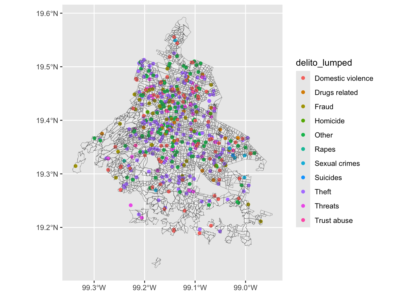

Now, I want to plot all the DV crimes on a map, to examine density, irrespective of which AGEB it falls in. Basically, a dot-density map, only for a year, so that we still see sth.

The large AGEB with no crimes are like airport, highways, etc. I checked and population is very low in these AGEBs.

ggplot() +
  geom_sf(data = carpetas %>% filter(delito_lumped == "Domestic violence") %>% filter(year(date)==2018),
          size = 0.1,
          color = "red",
          alpha = .5) +
  geom_sf(data = ageb, fill = NA, linewidth = .1) +
  annotation_scale(location = "br", style = "ticks") +
  theme_map()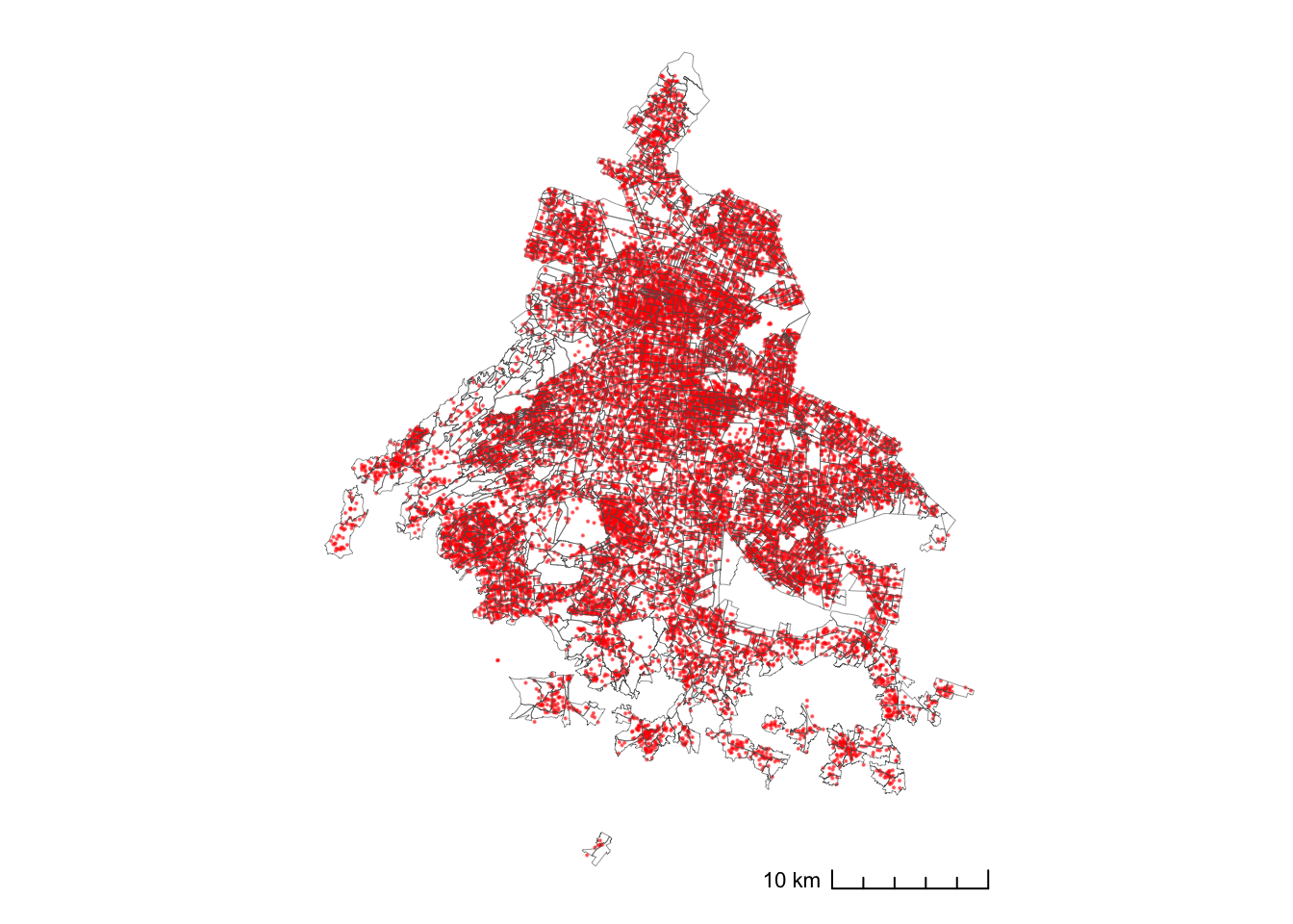 

Assign the crime incidents to a AGEB

I want to know in which AGEB each crime took place. To that end, I spatially join the two datasets, i.e. I compare each crime’s location to the polygons that represent the AGEBs.

I perform an inner join, because I only want to keep the crime reports located within CMDX.

carpetas <- 
  st_join(carpetas, ageb,
          left = FALSE) # inner join

Now, I keep only the AGEB identifier to identify the location.

carpetas <- carpetas %>% 
  select(-alcaldia_hecho, -alcaldia_catalogo, -municipio_hecho,
         -colonia_hecho, -colonia_catalogo) %>% 
  st_drop_geometry() %>% 
  as_tibble()

7 Save the cleaned crime data

Save the cleaned crime-level data, still contains all types of crime

carpetas %>% 
  write_rds(here("..",
               "output",
               "temporary_data",
               "dv",
               "PGJ_carpetas.rds"))

8 Plot the data

carpetas <-  
  read_rds(here("..",
               "output",
               "temporary_data",
               "dv",
               "PGJ_carpetas.rds"))

Select pre-covid

# carpetas <- carpetas %>% 
#   filter(year(date) < 2020)

Plot distribution over time

carpetas %>% 
  filter(delito_lumped == "Domestic violence") %>% 
  mutate(Date = decimal_date(date)) %>% 
  count(Date) %>% 
  ggplot() +
  geom_rect(data = data.frame(xmin = decimal_date(as.Date(c("2020-02-15"))),
                              xmax = decimal_date(as.Date(c("2021-11-01"))),
                              ymin = -Inf,
                              ymax = Inf),
            aes(xmin = xmin, xmax = xmax, ymin = ymin, ymax = ymax),
            fill = "red", alpha = 0.3) +
  geom_line(aes(Date, n), colour = "black", stat = 'identity') +
  scale_x_continuous(breaks = 2016:2024) +
  labs(x = element_blank(),
       y = "Daily reports for DV")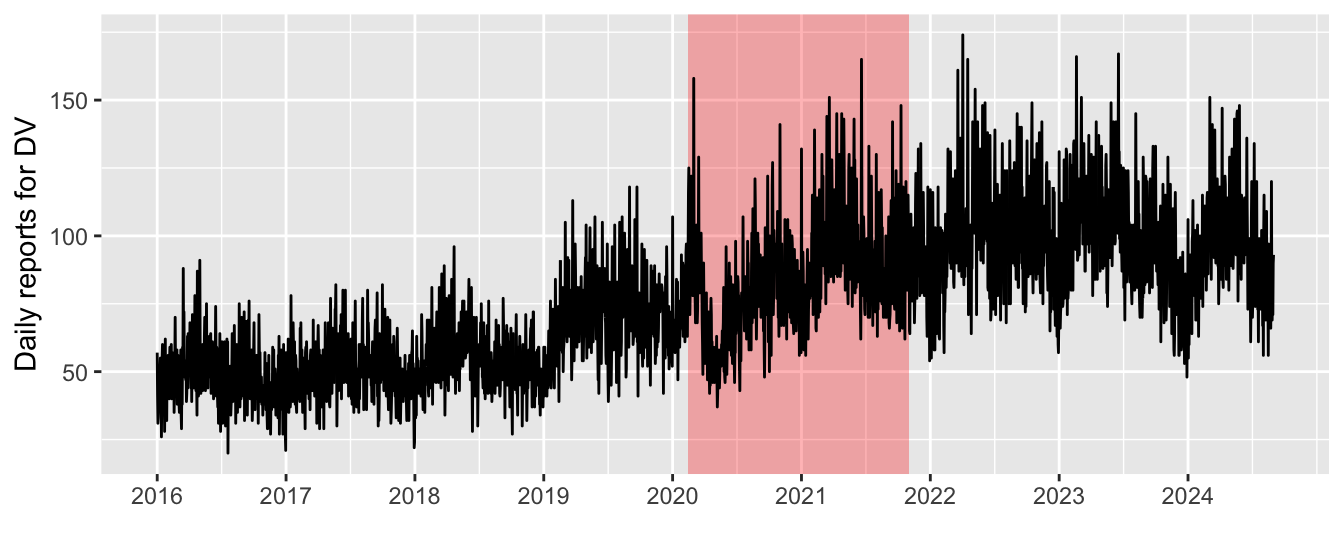 

Over the years

carpetas %>% 
  filter(delito_lumped == "Domestic violence") %>% 
  mutate(year = year(date)) %>%
  ggplot(aes(year)) +
  geom_bar() +
  scale_x_continuous(breaks = 2016:2024) +
  labs(x = element_blank(),
       y = element_blank())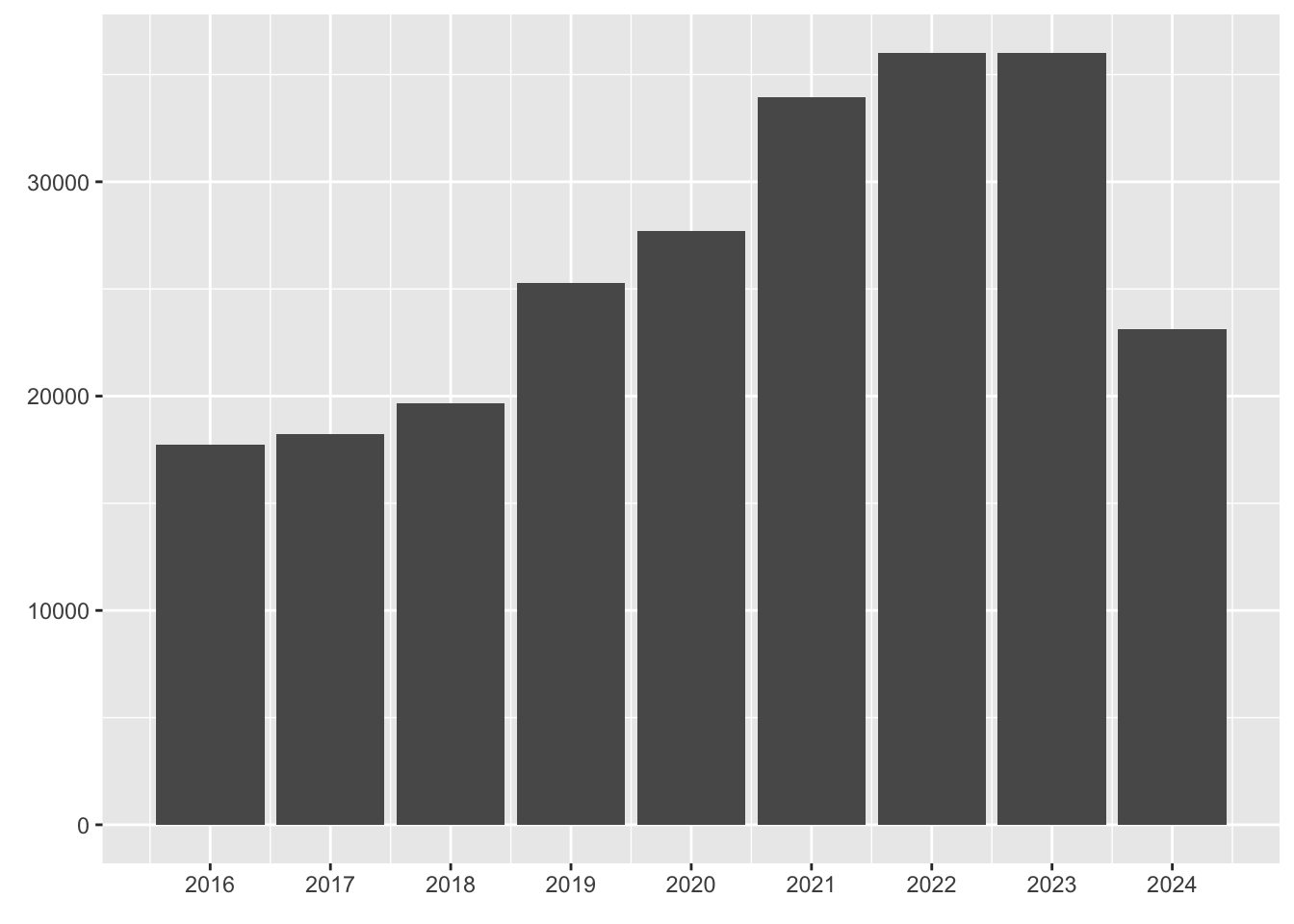

Over the months

carpetas %>%
  filter(delito_lumped == "Domestic violence") %>% 
  ggplot(aes(lubridate::month(date, label = T))) +
  geom_bar()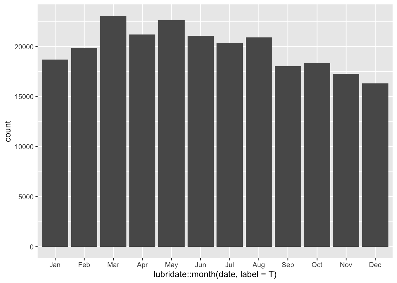

2020 is really the weird one: covid

carpetas %>%
  filter(delito_lumped == "Domestic violence") %>% 
  count(Year = as_factor(year(date)), Month = lubridate::month(date, label = T)) %>% 
  ggplot(aes(Month, n,
             group = Year, color = Year)) +
  geom_line()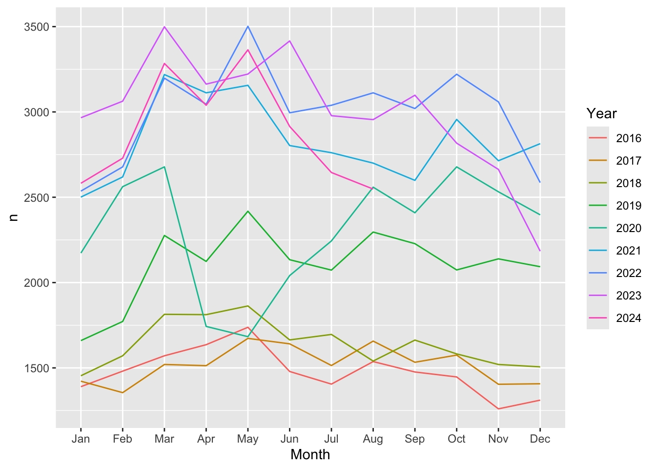

There a clear increase of DV cases recorded over time, going from less than 1,500 monthly cases per month in 2016 to more than 3,000 in 2022.

carpetas %>%
  filter(delito_lumped == "Domestic violence") %>% 
  count(Year = as_factor(year(date)),
        Month = lubridate::month(date, label = T)) %>% 
  ggplot(aes(Month, n, group = Year)) +
  geom_line() +
  facet_grid(~ Year) +
  scale_x_discrete(labels = NULL) +
  labs(x = "", y = "Monthly DV reports",
       title = "Total number of DV cases per month by year")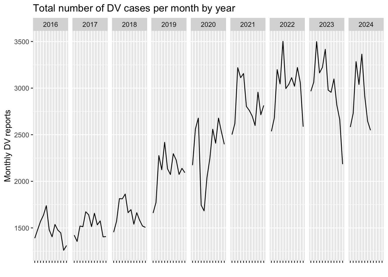 

Over the days of the week

carpetas %>% 
  filter(delito_lumped == "Domestic violence") %>% 
  ggplot(aes(x = lubridate::wday(date, label = T, week_start = 1))) +
  geom_bar() +
  labs(x = element_blank(),
       y = element_blank())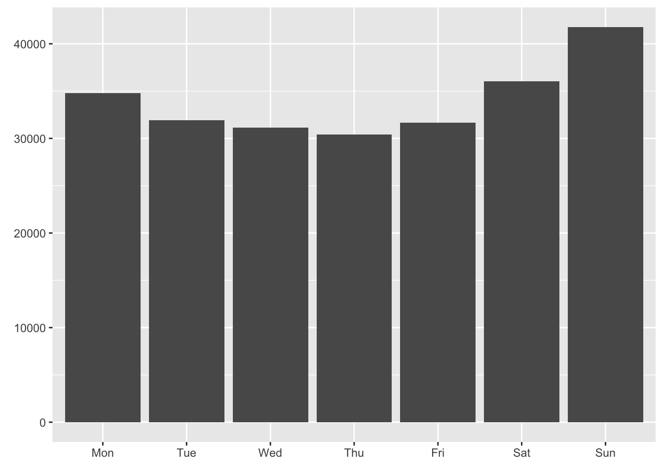

Over the hours of the day

carpetas %>% 
  filter(delito_lumped == "Domestic violence") %>% 
  ggplot(aes(x = hour(dttm))) +
  geom_bar() +
  scale_x_continuous(breaks=0:23) +
  labs(x = element_blank(),
       y = element_blank())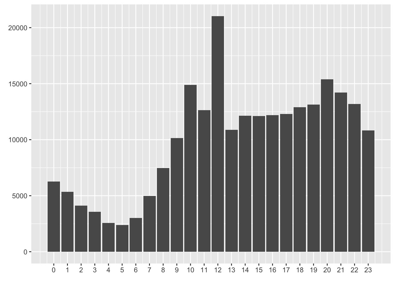

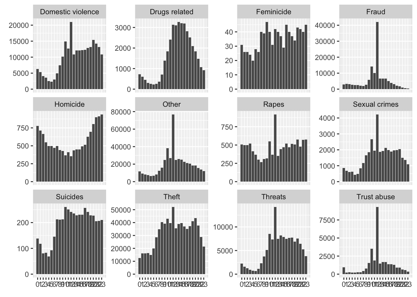
Now, facet for the different types of crime. It gives us an idea of the quality of the data per crime.

carpetas %>% 
  ggplot(aes(x = hour(dttm))) +
  geom_bar() +
  scale_x_continuous(breaks=0:23) +
  labs(x = element_blank(),
       y = element_blank()) +
  facet_wrap(~delito_lumped, scales = "free_y")