Robustness

Note

I run all the robustness/sensitivity checks here.

weekend vs weekdays
weather controls (add and remove them)
pre-post pandemic
Aggregate at mun level
Set of fixed effects
Sample split by day of week

start_time <- Sys.time()

library(tidyverse)
library(here) # path control
library(fixest) # estimations with fixed effects
library(knitr)
library(tictoc)
tic("Total render time")

source("fun_dynamic_bins.R")

mem.maxVSize(vsize = 40000)

[1] 40000

Import the full data to test pre-post pandemic and also the pre-pandemic data.

data_full <-
  read_rds(here("..", "output", "data_reports.rds"))

data_full <- data_full %>% 
  mutate(prec_quintile = ntile(prec, 5),
         rh_quintile = ntile(rh, 5),
         wsp_quintile = ntile(wsp, 5))

data <-
  read_rds(here("..", "output", "data_reports.rds")) %>% 
  filter(covid_phase == "Pre-pandemic")

data <- data %>% 
  mutate(prec_quintile = ntile(prec, 5),
         rh_quintile = ntile(rh, 5),
         wsp_quintile = ntile(wsp, 5))

Pre, post, during PANDEMIC

Here are the pandemic phases. I don’t remember exactly how i defined it, but i researched it… Pretty useless now since i do pre pandemic only, but oh well

data_full %>% 
  distinct(date, covid_phase) %>%
  group_by(covid_phase) %>%
  summarise(nr_days = n(), min_date = min(date), max_date = max(date)) %>% 
  arrange(min_date) %>% 
  kable()

covid_phase	nr_days	min_date	max_date
Pre-pandemic	1506	2016-01-01	2020-02-14
Pandemic	625	2020-02-15	2021-10-31
Post-pandemic	1035	2021-11-01	2024-08-31

Look at share of missing variables per phase (in pc), we have very few and not more in old data than in new one.

data_full %>%
  select(reports_dv, tmean,
         prec_quintile, rh_quintile, wsp_quintile,
         covid_phase) %>% 
  group_by(covid_phase) %>% 
  summarise(across(everything(), ~ 100*sum(is.na(.)/n()))) %>% 
  kable()

covid_phase	tmean	prec_quintile	rh_quintile	wsp_quintile
Pandemic	0.0146892	0.0000000	0.0214739	0.0058625
Post-pandemic	0.1003574	0.1932367	0.1014712	0.1057671
Pre-pandemic	0.0016949	0.0000000	0.0028704	0.0009295

Run the regressions:

reg_baseline <- data_full %>% 
  filter(covid_phase == "Pre-pandemic") %>% 
  fepois(reports_dv ~ tmean |
           prec_quintile + rh_quintile + wsp_quintile +
           ageb + year^month + day_of_week + day_of_year,
         cluster = ~ ageb)

reg_pandemic <- data_full %>% 
  filter(covid_phase == "Pandemic") %>% 
  fepois(reports_dv ~ tmean |
           prec_quintile + rh_quintile + wsp_quintile +
           ageb + year^month + day_of_week + day_of_year,
         cluster = ~ ageb)

reg_post <- data_full %>% 
  filter(covid_phase == "Post-pandemic") %>% 
  fepois(reports_dv ~ tmean |
           prec_quintile + rh_quintile + wsp_quintile +
           ageb + year^month + day_of_week + day_of_year,
         cluster = ~ ageb)


reg_all_periods <- data_full %>% 
  fepois(reports_dv ~ tmean |
           prec_quintile + rh_quintile + wsp_quintile +
           ageb + year^month + day_of_week + day_of_year,
         cluster = ~ ageb)


etable(reg_baseline, reg_pandemic, reg_post, reg_all_periods) %>% 
  kable()

	reg_baseline	reg_pandemic	reg_post	reg_all_periods
Dependent Var.:	Reports	Reports	Reports	Reports

Temperature	0.0277*** (0.0034)	0.0345*** (0.0063)	0.0293*** (0.0035)	0.0263*** (0.0020)
Fixed-Effects:	——————	——————	——————	——————
Precipitation	Yes	Yes	Yes	Yes
Humidity	Yes	Yes	Yes	Yes
Windspeed	Yes	Yes	Yes	Yes
Neighborhood	Yes	Yes	Yes	Yes
Year-Month	Yes	Yes	Yes	Yes
Day of Week	Yes	Yes	Yes	Yes
Day of Year	Yes	Yes	Yes	Yes
_______________	__________________	__________________	__________________	__________________
S.E.: Clustered	by: Neighborhood	by: Neighborhood	by: Neighborhood	by: Neighborhood
Observations	3,624,826	1,496,546	2,495,039	7,675,815
Squared Cor.	0.01332	0.02135	0.02330	0.01988
Pseudo R2	0.05611	0.06577	0.06779	0.06633
BIC	804,228.9	472,305.8	838,987.7	2,047,300.0

rm(data_full)

Weekend vs weekdays

Interact tmean with the weekend dummy

reg_weekend_interacted <- data %>%
  fepois(reports_dv ~ i(weekend_dummy, tmean) |
           prec_quintile + rh_quintile + wsp_quintile +
           ageb + year^month + day_of_year,
         cluster = ~ ageb)

etable(reg_weekend_interacted) %>% 
  kable()

	reg_weekend_inte..
Dependent Var.:	Reports

Temperature x weekend_dummy = Weekdays	0.0258*** (0.0034)
Temperature x weekend_dummy = Weekend	0.0351*** (0.0034)
Fixed-Effects:	——————
Precipitation	Yes
Humidity	Yes
Windspeed	Yes
Neighborhood	Yes
Year-Month	Yes
Day of Year	Yes
______________________________________	__________________
S.E.: Clustered	by: Neighborhood
Observations	3,624,826
Squared Cor.	0.01323
Pseudo R2	0.05586
BIC	804,354.3

wald(reg_weekend_interacted, "weekend_dummy::Weekend:tmean = weekend_dummy::Weekdays:tmean")

[1] NA

library(car)
linearHypothesis(reg_weekend_interacted, "weekend_dummy::Weekend:tmean = weekend_dummy::Weekdays:tmean")


Linear hypothesis test:
- weekend_dummy::Weekdays:tmean  + weekend_dummy::Weekend:tmean = 0

Model 1: restricted model
Model 2: reports_dv ~ i(weekend_dummy, tmean) | prec_quintile + rh_quintile + 
    wsp_quintile + ageb + year^month + day_of_year

   Res.Df Df  Chisq Pr(>Chisq)    
1 3621992                         
2 3621991  1 347.25  < 2.2e-16 ***
---
Signif. codes:  0 '***' 0.001 '**' 0.01 '*' 0.05 '.' 0.1 ' ' 1

Weather controls

I first want to look at the quintiles of the weather controls, how the distributions and thresholds look like.

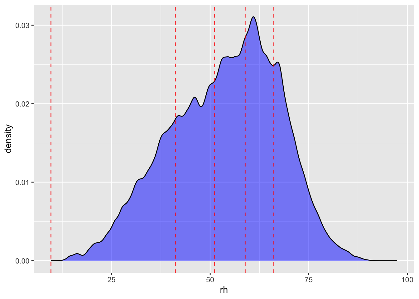
First look at humidity:

rh_quintile	mean(rh)	min(rh)	max(rh)
1	33.41955	9.620559	41.16997
2	46.31724	41.169972	51.10548
3	55.07531	51.105494	58.86866
4	62.29112	58.868661	65.98551
5	71.56685	65.985516	97.41922
NA	NA	NA	NA

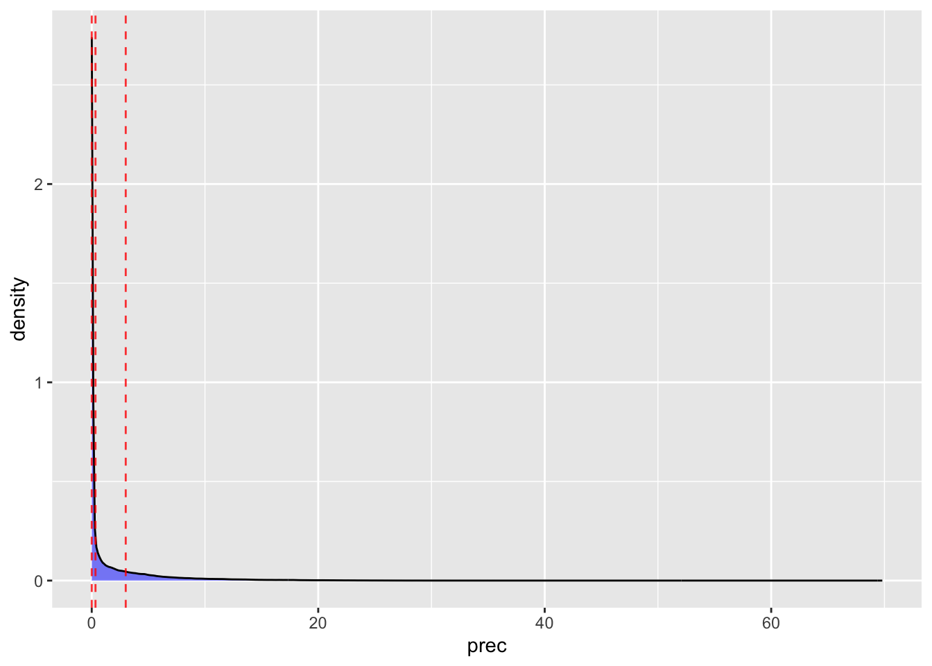
Precipitation

prec_quintile	mean(prec)	min(prec)	max(prec)
1	0.0000000	0.0000000	0.0000000
2	0.0000000	0.0000000	0.0000000
3	0.0783131	0.0000000	0.3326569
4	1.3807250	0.3326613	3.0022805
5	7.9591730	3.0022835	69.8145571

and windspeed

wsp_quintile	mean(wsp)	min(wsp)	max(wsp)
1	1.550543	0.8699148	1.720393
2	1.830580	1.7203941	1.931157
3	2.025840	1.9311576	2.127878
4	2.263310	2.1278780	2.425654
5	2.836775	2.4256551	9.170833
NA	NA	NA	NA

Now, run some regs

entering controls linearly instead of quintiles
excluding them altogether
only including one at a time

reg_weather_controls_linear <- data %>% 
  fepois(reports_dv ~ tmean + prec + rh + wsp |
           #prec_quintile + rh_quintile + wsp_quintile +
           ageb + year^month + day_of_week + day_of_year,
         cluster = ~ ageb)

reg_no_weather_controls <- data %>% 
  fepois(reports_dv ~ tmean |
           #prec_quintile + rh_quintile + wsp_quintile +
           ageb + year^month + day_of_week + day_of_year,
         cluster = ~ ageb)

reg_only_prec <- data %>% 
  fepois(reports_dv ~ tmean |
           prec_quintile +
           ageb + year^month + day_of_week + day_of_year,
         cluster = ~ ageb)

reg_only_rh <- data %>% 
  fepois(reports_dv ~ tmean |
           rh_quintile +
           ageb + year^month + day_of_week + day_of_year,
         cluster = ~ ageb)

reg_only_wsp <- data %>% 
  fepois(reports_dv ~ tmean |
           wsp_quintile +
           ageb + year^month + day_of_week + day_of_year,
         cluster = ~ ageb)

etable(reg_baseline,
       reg_no_weather_controls,
       reg_only_prec, reg_only_rh, reg_only_wsp) %>% 
  kable()

	reg_baseline	reg_no_weather_c..	reg_only_prec	reg_only_rh	reg_only_wsp
Dependent Var.:	Reports	Reports	Reports	Reports	Reports

Temperature	0.0277*** (0.0034)	0.0335*** (0.0027)	0.0307*** (0.0029)	0.0285*** (0.0033)	0.0332*** (0.0028)
Fixed-Effects:	——————	——————	——————	——————	——————
Precipitation	Yes	No	Yes	No	No
Humidity	Yes	No	No	Yes	No
Windspeed	Yes	No	No	No	Yes
Neighborhood	Yes	Yes	Yes	Yes	Yes
Year-Month	Yes	Yes	Yes	Yes	Yes
Day of Week	Yes	Yes	Yes	Yes	Yes
Day of Year	Yes	Yes	Yes	Yes	Yes
_______________	__________________	__________________	__________________	__________________	__________________
S.E.: Clustered	by: Neighborhood	by: Neighborhood	by: Neighborhood	by: Neighborhood	by: Neighborhood
Observations	3,624,826	3,624,883	3,624,883	3,624,826	3,624,883
Squared Cor.	0.01332	0.01332	0.01332	0.01333	0.01332
Pseudo R2	0.05611	0.05608	0.05609	0.05611	0.05609
BIC	804,228.9	804,080.1	804,128.4	804,115.2	804,134.4

Export the table as reg_weather_controls.tex

Aggregate at mun level

I aggregate the data at the municipality level, only 16 in mexico city. I weight by population size of AGEB.

data_mun <- data %>% 
  left_join(read_rds(here("..", "output", "ageb_attributes.rds")) %>% 
              select(ageb, nom_mun, pobtot),
            by = "ageb") %>%
  group_by(nom_mun, date) %>% 
  summarise(reports_dv = sum(reports_dv, na.rm = TRUE),
            tmean = weighted.mean(tmean, pobtot, na.rm = TRUE),
            prec = weighted.mean(prec, pobtot, na.rm = TRUE),
            rh = weighted.mean(rh, pobtot, na.rm = TRUE),
            wsp = weighted.mean(wsp, pobtot, na.rm = TRUE),
            year = first(year),
            month = first(month),
            day_of_week = first(day_of_week),
            day_of_year = first(day_of_year),
            covid_phase = first(covid_phase)
  ) %>% 
  ungroup() %>% 
  mutate(prec_quintile = ntile(prec, 5),
         rh_quintile = ntile(rh, 5),
         wsp_quintile = ntile(wsp, 5))

reg_mun <- data_mun %>% 
  fepois(reports_dv ~ tmean |
           prec_quintile + rh_quintile + wsp_quintile +
           nom_mun + year^month + day_of_week + day_of_year,
         cluster = ~ nom_mun)

etable(reg_baseline, reg_mun) %>% 
  kable()

	reg_baseline	reg_mun
Dependent Var.:	Reports	Reports

Temperature	0.0277*** (0.0034)	0.0259*** (0.0048)
Fixed-Effects:	——————	——————
Precipitation	Yes	Yes
Humidity	Yes	Yes
Windspeed	Yes	Yes
Neighborhood	Yes	No
Year-Month	Yes	Yes
Day of Week	Yes	Yes
Day of Year	Yes	Yes
nom_mun	No	Yes
_______________	__________________	__________________
S.E.: Clustered	by: Neighborhood	by: nom_mun
Observations	3,624,826	24,096
Squared Cor.	0.01332	0.60480
Pseudo R2	0.05611	0.27008
BIC	804,228.9	97,831.6

Sample split by day of week

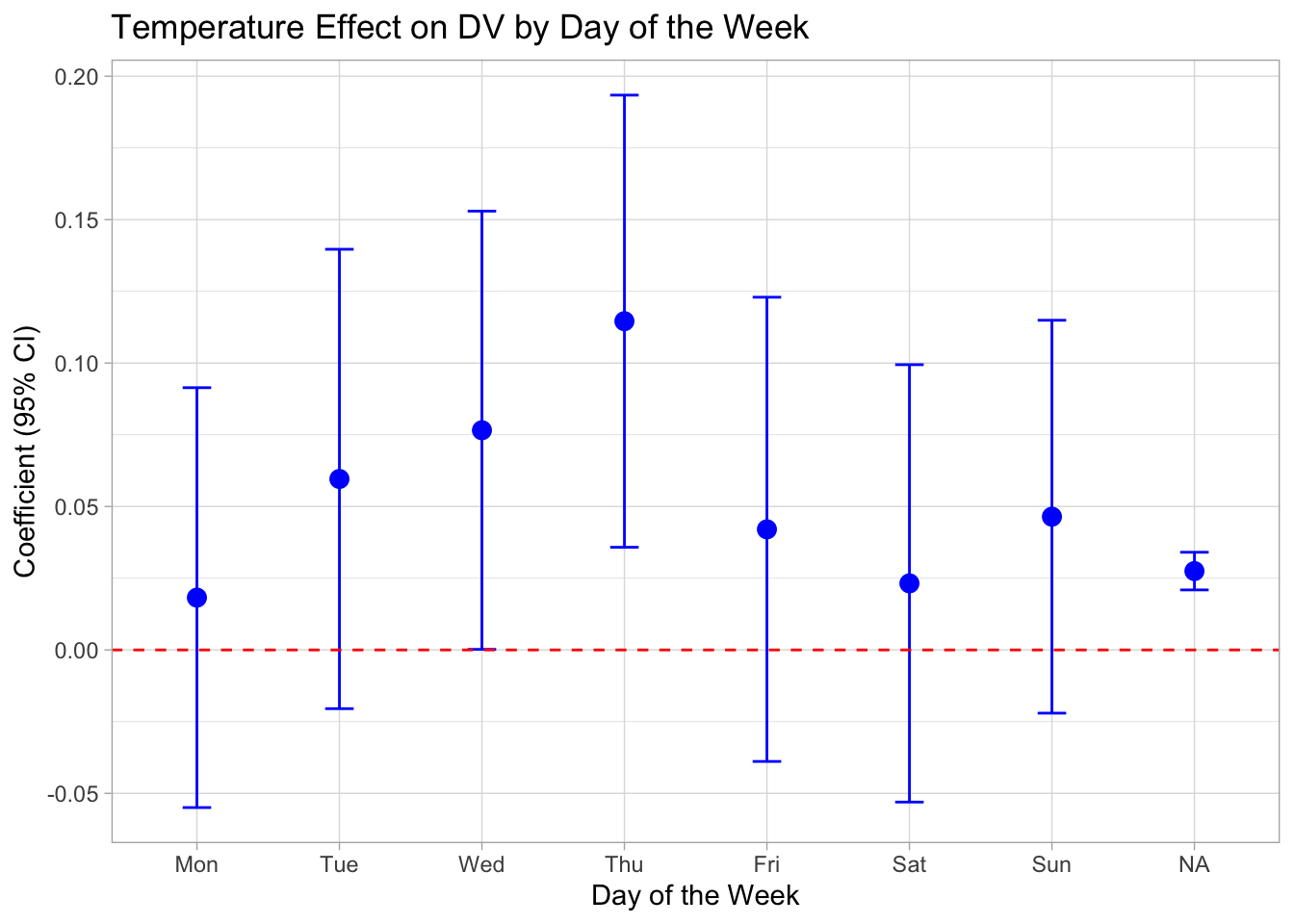
Since removing the FE for day of week makes little difference, I run a sample split for each day. There is not much happening there….

reg_split_day_of_week <- data %>% 
  fepois(reports_dv ~ tmean |
           prec_quintile + rh_quintile + wsp_quintile +
           ageb + year^month + day_of_year, 
         cluster = ~ ageb,
         fsplit = ~ day_of_week)

Note, its fsplit so estimate for NA is for the full sample.

Set of fixed effects

I try with different sets of fixed effects. This takes forever…

reg_fe_no_neighborhood <- data %>% 
  fepois(reports_dv ~ tmean |
           prec_quintile + rh_quintile + wsp_quintile +
           year^month + day_of_week + day_of_year,
         cluster = ~ ageb)

# reg_fe_no_temporal <- data %>% 
#   filter(covid_phase == "Pre-pandemic") %>% 
#   fepois(reports_dv ~ tmean |
#            prec_quintile + rh_quintile + wsp_quintile +
#            ageb, #+ year^month + day_of_week + day_of_year,
#          cluster = ~ ageb)

reg_fe_drop_year <- data %>% 
  fepois(reports_dv ~ tmean |
           prec_quintile + rh_quintile + wsp_quintile +
           ageb + month + day_of_week + day_of_year,
         cluster = ~ ageb)

reg_fe_drop_month <- data %>% 
  fepois(reports_dv ~ tmean |
           prec_quintile + rh_quintile + wsp_quintile +
           ageb + year + day_of_week + day_of_year,
         cluster = ~ ageb)

reg_fe_drop_month_and_doy <- data %>% 
  fepois(reports_dv ~ tmean |
           prec_quintile + rh_quintile + wsp_quintile +
           ageb + year + day_of_week, # + day_of_year + month
         cluster = ~ ageb)

reg_fe_drop_doy <- data %>% 
  fepois(reports_dv ~ tmean |
           prec_quintile + rh_quintile + wsp_quintile +
           ageb + year^month + day_of_week, # + day_of_year,
         cluster = ~ ageb)

reg_fe_drop_dow <- data %>% 
  fepois(reports_dv ~ tmean |
           prec_quintile + rh_quintile + wsp_quintile +
           ageb + year^month + day_of_year,# + day_of_week + ,
         cluster = ~ ageb)

etable(reg_baseline,
       reg_fe_no_neighborhood,
       reg_fe_drop_month,
       reg_fe_drop_doy,
       reg_fe_drop_month_and_doy,
       reg_fe_drop_dow) %>% 
  kable()

	reg_baseline	reg_fe_no_neig..	reg_fe_drop_month	reg_fe_drop_doy	reg_fe_drop_mont..	reg_fe_drop_dow
Dependent Var.:	Reports	Reports	Reports	Reports	Reports	Reports

Temperature	0.0277*** (0.0034)	0.0141* (0.0062)	0.0245*** (0.0031)	0.0285*** (0.0029)	0.0348*** (0.0019)	0.0275*** (0.0033)
Fixed-Effects:	——————	—————-	——————	——————	——————	——————
Precipitation	Yes	Yes	Yes	Yes	Yes	Yes
Humidity	Yes	Yes	Yes	Yes	Yes	Yes
Windspeed	Yes	Yes	Yes	Yes	Yes	Yes
Neighborhood	Yes	No	Yes	Yes	Yes	Yes
Year-Month	Yes	Yes	No	Yes	No	Yes
Day of Week	Yes	Yes	Yes	Yes	Yes	No
Day of Year	Yes	Yes	Yes	No	No	Yes
Year	No	No	Yes	No	Yes	No
_______________	__________________	________________	__________________	__________________	__________________	__________________
S.E.: Clustered	by: Neighborhood	by: Neighborhood	by: Neighborhood	by: Neighborhood	by: Neighborhood	by: Neighborhood
Observations	3,624,826	3,657,955	3,624,826	3,624,826	3,624,826	3,624,826
Squared Cor.	0.01332	0.00116	0.01328	0.01304	0.01297	0.01306
Pseudo R2	0.05611	0.00533	0.05596	0.05531	0.05509	0.05539
BIC	804,228.9	810,383.2	803,673.4	799,365.0	798,861.1	804,720.5

Export the table as reg_varying_fixef.tex

Modelling the LHS

If I do ols, i will need this in the table

# and a function computing the effect size in pc(i.e. 100*temp coef/mean DV)
my_fun_effsize_1 =
  function(x) paste0(round(
    100*coef(x)[1]/mean(model.matrix(x, type = "lhs")), 2),"%")
extralines_register("tmean_eff_size_1", my_fun_effsize_1, "__Effect size (1)")

my_fun_effsize_2 =
  function(x) ifelse(is.na(coef(x)[2]),
                     "--",
                     paste0(round(100*coef(x)[2]/mean(model.matrix(x, type = "lhs")), 2),"%"))
extralines_register("tmean_eff_size_2", my_fun_effsize_2, "__Effect size (2)")

Rendered on: 2025-07-27 02:04:27

Total render time: 563.847 sec elapsed