Reporting bias

Note

I run all the analyses on the reporting bias.

start_time <- Sys.time()

library(tidyverse)
library(here) # path control
library(lubridate) # handle dates
library(fixest) # estimations with fixed effects
library(sf)
library(viridis)
library(tictoc)
library(knitr)
tic("Total render time")

Prepare the data

Load crime level data

carpetas <-  
  readRDS(here("..", "output",
               "temporary_data",
               "dv",
               "PGJ_carpetas.rds")) %>% 
  sf::st_drop_geometry() 

carpetas <- carpetas %>% 
  select(-c_id, #crime id, we keep ageb
         -latitud, -longitud) %>% 
  rename(dttm_hecho = dttm, fecha_hecho = date)

carpetas <- carpetas %>% 
  filter(delito_lumped == "Domestic violence") %>% 
  # recompute the deciles for DV crimes only
  mutate(decile_delay_full_days = ntile(delay_full_days, 10))

Join weather, both on crime day and reporting day

weather <-
  read_rds(here("..", "output", "temporary_data", "weather", "weather_cdmx.rds")) %>% 
  mutate(date = ymd(date)) %>% 
  select(ageb, date, tmean, prec_quintile, rh_quintile, wsp_quintile) 

# join the weather variables for day of crime
data <- left_join(carpetas, weather, by = c("fecha_hecho" = "date", "ageb"))
rm(carpetas)

# join the weather variables for day of report
weather <- weather %>% 
  #append all variables names with _report_day
  rename_with(~str_c(., "_report_day")) %>% 
  rename(fecha_inicio = date_report_day,
         ageb = ageb_report_day)

data <- left_join(data, weather, by = c("fecha_inicio", "ageb")) %>% 
  relocate(ageb, fecha_hecho, fecha_inicio, tmean, tmean_report_day)

rm(weather)

Filter and make FEs

#filter to pre pandemix, like the rest
data <- data %>%
  filter(fecha_hecho <= ymd("2020-02-14"))
# i also filter out the whole of 2020, because we look into the future
data <- data %>%
  filter(year(fecha_hecho) != 2020)


#Create a few variables for fixed effects
data <- data %>%
  mutate(year = lubridate::year(fecha_hecho),
         month = lubridate::month(fecha_hecho, label = T),
         day_of_week = lubridate::wday(fecha_hecho, label = TRUE),
         day_of_year = lubridate::yday(fecha_hecho))

Hours of crime

Hour cannot really be trusted… because of the 12:00 peak, but wihtout it, it seems OK.

# Extract hour hecho
data <- data %>%
  mutate(hour_hecho = as_factor(hour(dttm_hecho))) 

data %>% count(hour_hecho) %>% 
  ggplot(aes(hour_hecho, n)) +
  geom_col()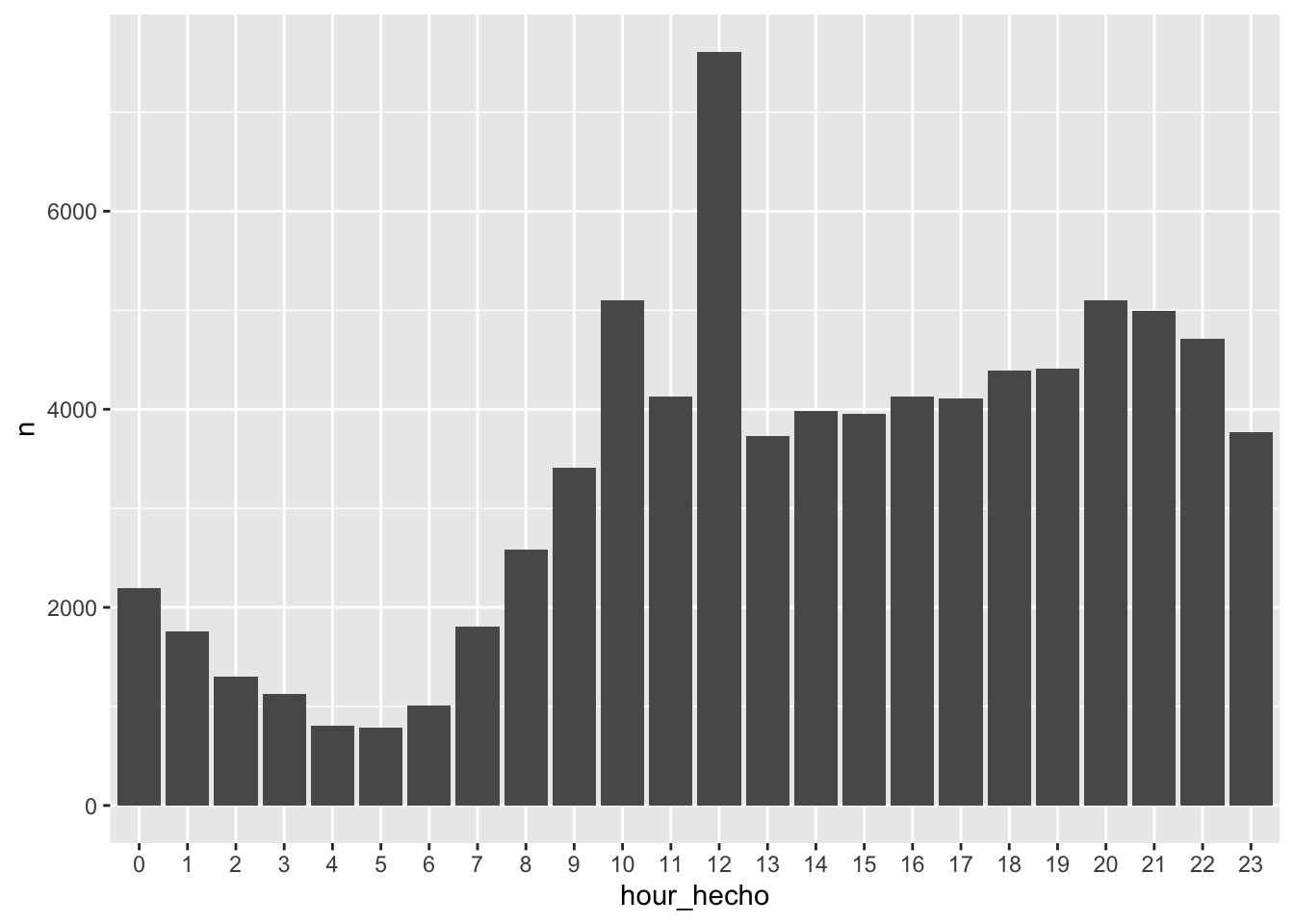

Take the log of delay+1 to dampen outliers

data <- data %>% 
  mutate(log_delay_full_days = log(delay_full_days + 1),
         log_delay_hours = log(delay_hours))

Create indicators for delay

data <- data %>%
  mutate(
    delay_zero = delay_full_days == 0,  # Indicator for zero delay
    delay_zero_or_one = delay_full_days %in% 0:1,  # Indicator for zero delay
    delay_positive = ifelse(delay_full_days > 0, delay_full_days, NA)  # Positive delays
  )

data %>% count(delay_full_days, delay_zero, delay_zero_or_one, delay_positive) %>% 
  head(10) %>%
  kable()

delay_full_days	delay_zero	delay_zero_or_one	delay_positive	n
0	TRUE	TRUE	NA	24976
1	FALSE	TRUE	1	19737
2	FALSE	FALSE	2	6553
3	FALSE	FALSE	3	4285
4	FALSE	FALSE	4	2767
5	FALSE	FALSE	5	1942
6	FALSE	FALSE	6	1503
7	FALSE	FALSE	7	1152
8	FALSE	FALSE	8	913
9	FALSE	FALSE	9	863

Describe the data

Long tails for the delays…

Distribution of delays (only most frequent)

data %>% 
  mutate(delay_full_days = if_else(delay_full_days > 56, 56, delay_full_days)) %>%
  count(delay_full_days) %>% 
  mutate(share = n/sum(n)) %>% 
  head(11) %>% kable()

delay_full_days	n	share
0	24976	0.3086467
1	19737	0.2439045
2	6553	0.0809802
3	4285	0.0529529
4	2767	0.0341938
5	1942	0.0239987
6	1503	0.0185737
7	1152	0.0142361
8	913	0.0112826
9	863	0.0106647
10	743	0.0091818

Min and max per decile

data %>% 
  group_by(decile_delay_full_days) %>% 
  summarise(min = min(delay_full_days),
            max = max(delay_full_days),
            mean = mean(delay_full_days),
            n = n()) %>% 
  kable()

decile_delay_full_days	min	max	mean	n
1	0	0	0.000000	23772
2	0	0	0.000000	1204
4	1	1	1.000000	19737
6	2	2	2.000000	6553
7	3	4	3.358341	6678
8	4	9	6.426412	6747
9	10	32	18.517083	8049
10	33	2939	161.661288	8181

Plot and save figure:

data <- data %>% 
  mutate(delay_full_days = if_else(delay_full_days >= 15, 15, delay_full_days)) %>%
  mutate(group_delay = case_when(
    decile_delay_full_days == 10 ~ "Top decile",
    delay_full_days == 0 ~ "Same day",
    delay_full_days == 1 ~ "Next day",
    delay_full_days <= 7 ~ "2-7 days",
    delay_full_days <= 14 ~ "8-14 days",
    delay_full_days >= 15 ~ ">14 days",
  ),
  group_delay = factor(group_delay, 
                       levels = c("Same day", "Next day", "2-7 days", "8-14 days", ">14 days", "Top decile"),
                       ordered = TRUE)
  )


data %>% 
  count(group_delay) %>% 
    mutate(prop = n / sum(n)) %>%
  ggplot(aes(x = group_delay, y = prop, fill = group_delay)) +
  geom_col() +
  scale_y_continuous(labels = scales::percent) +
  labs(x = NULL,
       y = NULL,
       fill = NULL) +
  scale_fill_manual(values = c("Same day" = viridis(9)[2],
                               "Next day" = viridis(9)[2],
                               "2-7 days" = viridis(9)[2],
                               "8-14 days" = viridis(9)[2],
                               ">14 days" = viridis(9)[2],
                               "Top decile" = "gray70")) +
  theme_light() +
  theme(legend.position = "none")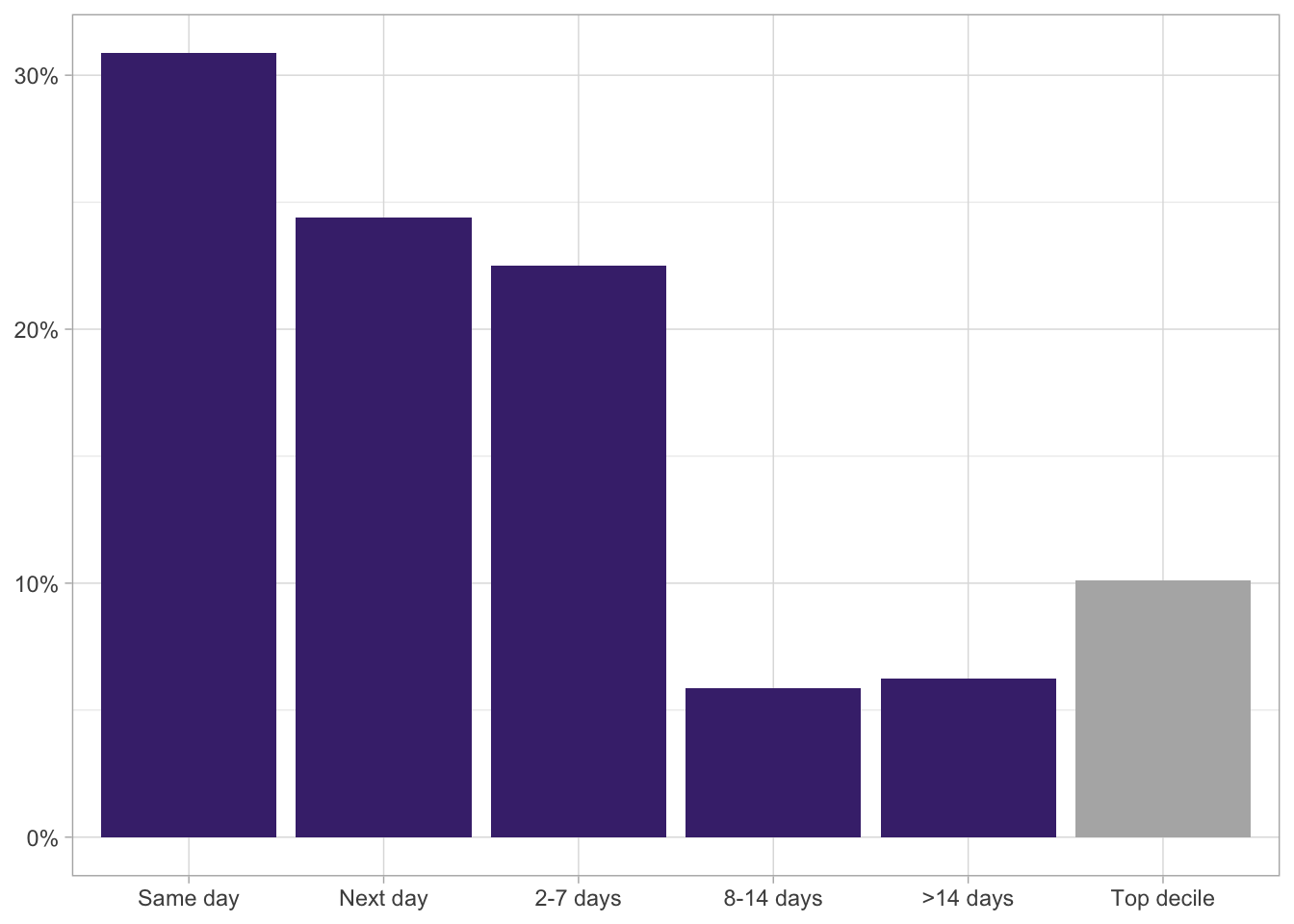

ggsave(here("..", "output", "figures", "reporting_delays_distrib.png"),
       width = 6, height = 3, dpi = 300)

Model the Reporting Delays

For both the logit and the negbin, i exclude the top decile of delays. There are many reasons:

• These very delayed reports are likely driven by retrospective or institutional processes (e.g., follow-ups, legal obligations) rather than immediate behavioral responses.
• Including them may introduce noise and weaken identification of any contemporaneous relationship between incident-day temperature and reporting behavior.
• The focus is on whether temperature affects promptness of reporting as a proxy for reporting incentives — long delays are conceptually distinct from that process.
• Trimming the top 10% improves model stability and keeps the analysis aligned with the paper’s main behavioral mechanism.

Model the Probability of same day report

logit_model <-
  data %>% 
  filter(decile_delay_full_days != 10) %>%
  feglm(delay_zero ~ tmean |
          prec_quintile + rh_quintile + wsp_quintile +
          ageb + year^month + day_of_week + day_of_year,
        family = binomial(link = "logit"),
        cluster = ~ ageb)

etable(logit_model) %>% 
  kable()

	logit_model
Dependent Var.:	delay_zero
tmean	0.0036 (0.0083)
Fixed-Effects:	—————
prec_quintile	Yes
rh_quintile	Yes
wsp_quintile	Yes
ageb	Yes
year-month	Yes
day_of_week	Yes
day_of_year	Yes
_______________	_______________
S.E.: Clustered	by: ageb
Observations	72,378
Squared Cor.	0.05175
Pseudo R2	0.04135
BIC	119,897.3

Model the Positive Delays

nb_model <- 
  data %>% 
  filter(decile_delay_full_days != 10) %>%
  filter(delay_full_days > 0) %>% 
  fenegbin(
  delay_positive ~ tmean |
    prec_quintile + rh_quintile + wsp_quintile +
    ageb + year^month + day_of_week + day_of_year,
  cluster = ~ ageb
)

nb_model_both <- 
  data %>% 
  filter(decile_delay_full_days != 10) %>%
  filter(delay_full_days > 0) %>% 
  fenegbin(
  delay_positive ~ tmean + tmean_report_day |
    prec_quintile + rh_quintile + wsp_quintile +
    ageb + year^month + day_of_week + day_of_year,
  cluster = ~ ageb
)

etable(nb_model, nb_model_both) %>% 
  kable()

	nb_model	nb_model_both
Dependent Var.:	delay_positive	delay_positive
tmean	-0.0124* (0.0061)	-0.0109. (0.0062)
tmean_report_day		-0.0117* (0.0046)
Fixed-Effects:	—————–	—————–
prec_quintile	Yes	Yes
rh_quintile	Yes	Yes
wsp_quintile	Yes	Yes
ageb	Yes	Yes
year-month	Yes	Yes
day_of_week	Yes	Yes
day_of_year	Yes	Yes
________________	_________________	_________________
S.E.: Clustered	by: ageb	by: ageb
Observations	47,764	47,764
Squared Cor.	0.07196	0.07177
Pseudo R2	0.02037	0.02041
BIC	286,414.9	286,413.8
Over-dispersion	1.1214	1.1216

Export the table for the two results above

etable(logit_model, nb_model, nb_model_both) %>% 
  kable()

	logit_model	nb_model	nb_model_both
Dependent Var.:	delay_zero	delay_positive	delay_positive
tmean	0.0036 (0.0083)	-0.0124* (0.0061)	-0.0109. (0.0062)
tmean_report_day			-0.0117* (0.0046)
Fixed-Effects:	—————	—————–	—————–
prec_quintile	Yes	Yes	Yes
rh_quintile	Yes	Yes	Yes
wsp_quintile	Yes	Yes	Yes
ageb	Yes	Yes	Yes
year-month	Yes	Yes	Yes
day_of_week	Yes	Yes	Yes
day_of_year	Yes	Yes	Yes
________________	_______________	_________________	_________________
Family	Logit	Neg. Bin.	Neg. Bin.
S.E.: Clustered	by: ageb	by: ageb	by: ageb
Observations	72,378	47,764	47,764
Squared Cor.	0.05175	0.07196	0.07177
Pseudo R2	0.04135	0.02037	0.02041
BIC	119,897.3	286,414.9	286,413.8
Over-dispersion	–	1.1214	1.1216

etable(logit_model, nb_model, nb_model_both,
       fitstat = ~ n,
       digits.stats = "s3", digits = "r4",
       #extralines = ~ tmean_eff_size_1 + tmean_eff_size_2,
       file = here(".." , "output", "tables", "reg_reporting_delays.tex"), replace = T,
       view = T,
       fixef_sizes = T,
       dict = c(ageb = "Neighborhood",
                tmean = "Temperature on incident day",
                tmean_report_day = "Temperature on reporting day",
                delay_zero = "Same day report",
                delay_positive = "Positive delay"),
       fixef.group=list("Prec, hum, wsp quintiles"="quintile",
                        "Date FEs"="month|day"),
       style.tex = style.tex("aer",
                             model.format = "(i)",
                             tpt = TRUE,
                             notes.tpt.intro = "\\footnotesize",
                             fixef.suffix = " FEs"),
       adjustbox = .8, float = T,
       title = "Temperature and Reporting Delays in DV Incidents",
       label = "reg_reporting_delays",
       notes = "Notes: Standard errors clustered by neighborhood in parentheses. * denotes significance at the 10% level, ** at the 5% level, and *** at the 1% level.
Incident level data. Incidents with a delay in the top decile (33+ days) are excluded from all estimations.
Column (i) reports the coefficient estimate from a logistic regression where the dependent variable is an indicator for same-day reporting.
Columns (ii) and (iii) report estimates from negative binomial models, estimated on the subsample of incidents reported with a delay of at least one day.
Column (ii) includes only temperature on the incident day; Column (iii) includes temperature on both the incident and reporting days.
All models year-month fixed effects, day-of-week fixed effects, and day-of-year fixed effects, controls for precipitation, humidity, and wind speed (in quintiles), and neighborhood fixed effects."
)

Use Reporting Time Categories as a Test for Reporting Bias

Disaggregate DV Reports by categories of delay

final_data <-
  read_rds(here("..", "output", "data_reports.rds")) %>% 
  filter(covid_phase == "Pre-pandemic")

final_data <- final_data %>% 
  mutate(prec_quintile = ntile(prec, 5),
         rh_quintile = ntile(rh, 5),
         wsp_quintile = ntile(wsp, 5))

final_data %>% 
  select(contains("reports_dv_delay")) %>% 
  names()

 [1] "reports_dv_delay_hours_[0-6]"    "reports_dv_delay_hours_(6-24]"  
 [3] "reports_dv_delay_hours_(24-48]"  "reports_dv_delay_hours_(48-168]"
 [5] "reports_dv_delay_hours_(168-)"   "reports_dv_delay_days_[0]"      
 [7] "reports_dv_delay_days_[1]"       "reports_dv_delay_days_[2-7]"    
 [9] "reports_dv_delay_days_[7-14]"    "reports_dv_delay_days_(14-)"    

#weird names fuck up the fixest estimations
final_data <- final_data %>% 
  rename_with(~ str_replace_all(., "[\\[\\]()]", "")) %>%  # Remove brackets and parentheses
  rename_with(~ str_replace_all(., "-", "_"))              # Replace dashes with underscores


reg_delays_days <- 
  fepois(c(reports_dv_delay_days_0,
           reports_dv_delay_days_1,
           reports_dv_delay_days_2_7,
           reports_dv_delay_days_7_14,
           reports_dv_delay_days_14_) ~ tmean |
           ageb + year^month + day_of_week + day_of_year +
           prec_quintile + rh_quintile + wsp_quintile,
         cluster = ~ ageb,
         data = final_data)

etable(reg_delays_days) %>% 
  kable()

	reg_delays_days.1	reg_delays_days.2	reg_delays_days.3	reg_delays_days.4	reg_delays_days.5
Dependent Var.:	reports_dv_delay_days_0	reports_dv_delay_days_1	reports_dv_delay_days_2_7	reports_dv_delay_days_7_14	reports_dv_delay_days_14_
tmean	0.0330*** (0.0061)	0.0327*** (0.0068)	0.0343*** (0.0070)	0.0233. (0.0132)	0.0044 (0.0078)
Fixed-Effects:	———————–	———————–	————————-	————————–	————————-
ageb	Yes	Yes	Yes	Yes	Yes
year-month	Yes	Yes	Yes	Yes	Yes
day_of_week	Yes	Yes	Yes	Yes	Yes
day_of_year	Yes	Yes	Yes	Yes	Yes
prec_quintile	Yes	Yes	Yes	Yes	Yes
rh_quintile	Yes	Yes	Yes	Yes	Yes
wsp_quintile	Yes	Yes	Yes	Yes	Yes
_______________	_______________________	_______________________	_________________________	__________________________	_________________________
S.E.: Clustered	by: ageb	by: ageb	by: ageb	by: ageb	by: ageb
Observations	3,490,792	3,454,648	3,453,142	2,784,491	3,383,869
Squared Cor.	0.00571	0.00427	0.00380	0.00121	0.00286
Pseudo R2	0.05462	0.04964	0.04783	0.03737	0.04464
BIC	331,391.6	279,985.1	264,939.3	104,175.2	212,956.0

etable(reg_delays_days,
       fitstat = ~ n + my,
       digits.stats = "s3", digits = "r4",
       #extralines = ~ tmean_eff_size_1 + tmean_eff_size_2,
       file = here("..", "output", "tables", "reg_reporting_delays_categories.tex"), replace = T,
       view = T,
       fixef_sizes = T,
       dict = c(ageb = "Neighborhood",
                tmean = "Temperature on incident day",
                tmean_report_day = "Temperature on reporting day",
                reports_dv_delay_days_0 = "Same day",
                reports_dv_delay_days_1 = "Next day",
                reports_dv_delay_days_2_7 = "2-7 days",
                reports_dv_delay_days_7_14 = "8-14 days",
                reports_dv_delay_days_14_ = ">14 days"),
       fixef.group=list("Prec, hum, wsp quintiles"="quintile",
                        "Date FEs"="month|day"),
       style.tex = style.tex("aer",
                             model.format = "(i)",
                             tpt = TRUE,
                             notes.tpt.intro = "\\footnotesize",
                             fixef.suffix = " FEs"),
       adjustbox = TRUE, float = T,
       title = "The Effect of Temperature on Reported DV by Delay in Reporting",
       label = "reg_reporting_delays_categories",
       notes = "Notes: Standard errors clustered by neighborhood in parentheses. * denotes significance at the 10% level, ** at the 5% level, and *** at the 1% level.
Dependent variable is the daily count of reported domestic violence incidents per neighborhood within each delay category.
Columns (i) through (v) report estimates from separate regressions, each estimated on a distinct subsample defined by reporting delay: same day, next day, 2–7 days, 8–14 days, and more than 14 days after the incident.
Year-month fixed effects, day-of-week fixed effects, and day-of-year fixed effects, controls for precipitation, humidity, and wind speed (in quintiles), and neighborhood fixed effects are included in each specification."
)

Rendered on: 2025-07-27 03:47:14

Total render time: 309.521 sec elapsed