I run the main regressions allowing for non-linear effects of temperature on domestic violence.
I estimate several regressions, with different binned temperature measures (tmean, tmax, tmin…)
I save plots for all the regs
For the main reg, with bins_tmean_one, I also
save a reg table for the main reg with tmean
compute summary statistics for the estimates
plot the support of bins and save it
<- Sys.time ()library (tidyverse)library (here) # path control library (fixest) # estimations with fixed effects library (modelsummary) # for the modelplot figure library (patchwork) # assemble the plots library (knitr) # for kable library (tictoc)tic ("Total render time" )source ("fun_dynamic_bins.R" )# Massive regressions, take ages to run, # set memory limit v high, also uses swap mem.maxVSize (vsize = 40000 )
<- read_rds (here (".." , "output" , "data_reports.rds" )) %>% filter (covid_phase == "Pre-pandemic" )<- data %>% mutate (prec_quintile = ntile (prec, 5 ),rh_quintile = ntile (rh, 5 ),wsp_quintile = ntile (wsp, 5 ))
Reports with bins_tmean_one
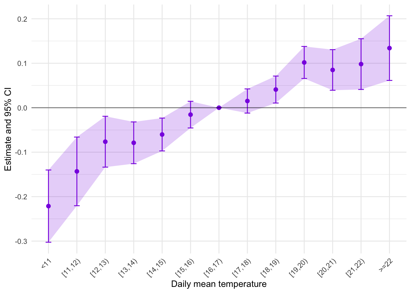
<- data %>% mutate (bins_tmean_one = create_dynamic_bins (tmean, width = 1 , 0.01 )) %>% fepois (reports_dv ~ i (bins_tmean_one, ref = "[16" ) | + rh_quintile + wsp_quintile + + year^ month + day_of_week + day_of_year,cluster = ~ ageb)
I can plot the estimates:
Or also show a table, and save it as reg_bins_reports.tex
Dependent Var.:
Reports
Daily Mean Temp. Bin = <11
-0.2227*** (0.0416)
Daily Mean Temp. Bin = [11,12)
-0.1427*** (0.0395)
Daily Mean Temp. Bin = [12,13)
-0.0767** (0.0293)
Daily Mean Temp. Bin = [13,14)
-0.0791*** (0.0240)
Daily Mean Temp. Bin = [14,15)
-0.0608** (0.0189)
Daily Mean Temp. Bin = [15,16)
-0.0165 (0.0154)
Daily Mean Temp. Bin = [17,18)
0.0143 (0.0139)
Daily Mean Temp. Bin = [18,19)
0.0396* (0.0155)
Daily Mean Temp. Bin = [19,20)
0.1005*** (0.0184)
Daily Mean Temp. Bin = [20,21)
0.0838*** (0.0233)
Daily Mean Temp. Bin = [21,22)
0.0971*** (0.0291)
Daily Mean Temp. Bin = >=22
0.1328*** (0.0371)
Fixed-Effects:
——————-
prec_quintile
Yes
rh_quintile
Yes
wsp_quintile
Yes
ageb
Yes
year-month
Yes
day_of_week
Yes
day_of_year
Yes
______________________________
___________________
S.E.: Clustered
by: ageb
Observations
3,624,826
Squared Cor.
0.01333
Pseudo R2
0.05613
BIC
804,379.5
I want to compute some summary stats:
<- iplot (reg_bins_reports, only.params = T)$ prms %>% as_tibble () %>% mutate (ref = estimate== 0 ) %>% left_join (data %>% count (estimate_names = create_dynamic_bins (tmean, width = 1 , 0.01 )) %>% mutate (share_in_pc = 100 * n / sum (n))) %>% #remove first and last, because its not a one degree jump slice (2 : (n () - 1 )) %>% select (estimate_names, estimate) %>% mutate (value_diff = estimate - lag (estimate),mean_diff = mean (value_diff, na.rm = T)) %>% kable ()
[11,12)
-0.1427025
NA
0.0239802
[12,13)
-0.0767282
0.0659743
0.0239802
[13,14)
-0.0791284
-0.0024002
0.0239802
[14,15)
-0.0607584
0.0183700
0.0239802
[15,16)
-0.0164686
0.0442898
0.0239802
[16,17)
0.0000000
0.0164686
0.0239802
[17,18)
0.0143096
0.0143096
0.0239802
[18,19)
0.0396283
0.0253187
0.0239802
[19,20)
0.1004997
0.0608714
0.0239802
[20,21)
0.0837827
-0.0167170
0.0239802
[21,22)
0.0970993
0.0133166
0.0239802
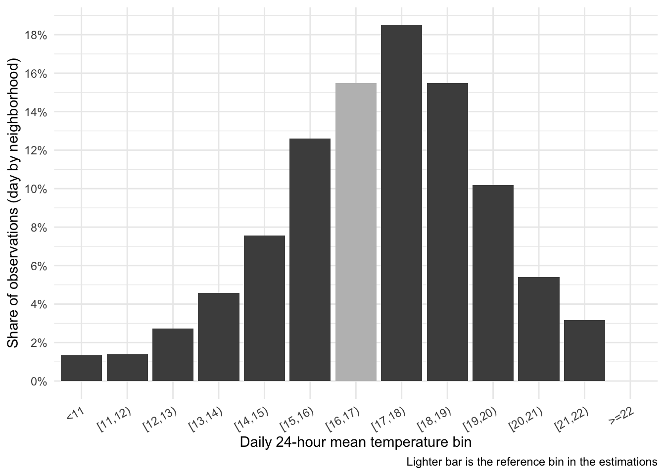
I also plot the support of the temp bins and save it as reg_bins_mean_temp_distrib.png
Reports with bins_tmax_one
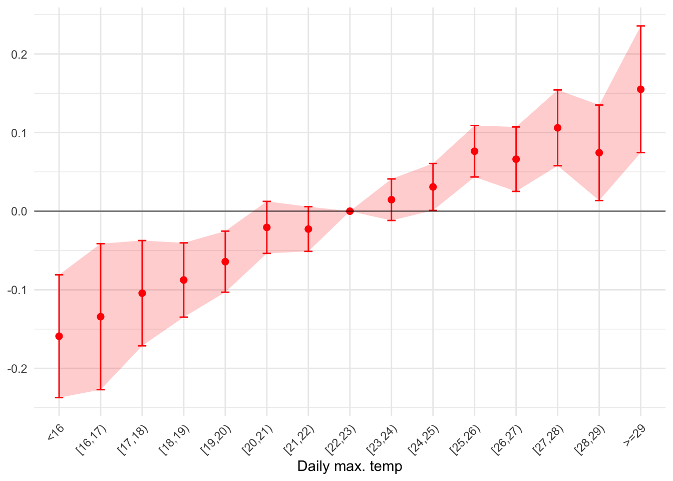
<- data %>% mutate (bins_tmax_one = create_dynamic_bins (tmax, width = 1 , 0.01 )) %>% fepois (reports_dv ~ i (bins_tmax_one, ref = "[22" ) | + rh_quintile + wsp_quintile + + year^ month + day_of_week + day_of_year,cluster = ~ ageb)
Plot and save as reg_bins_reports_tmax_1C.png
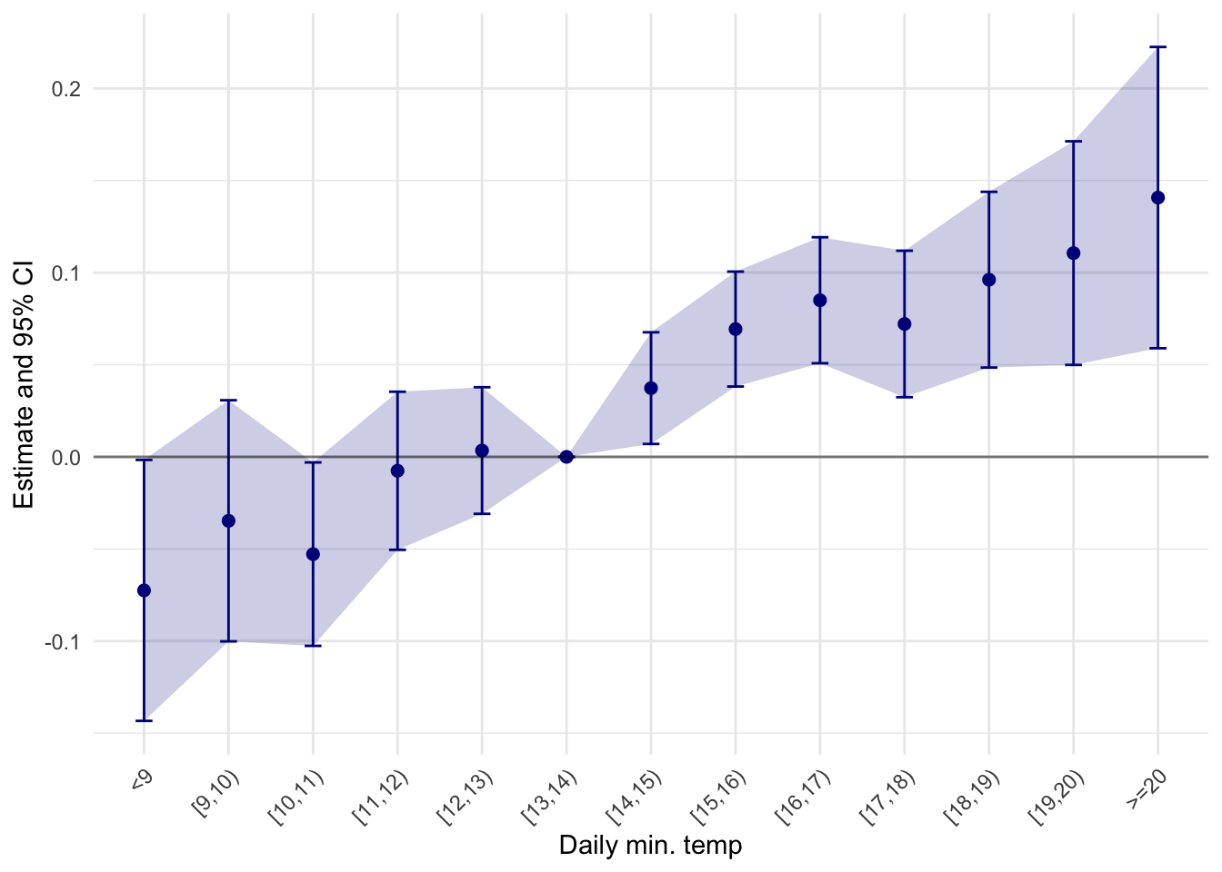
Reports with bins_tmin_one
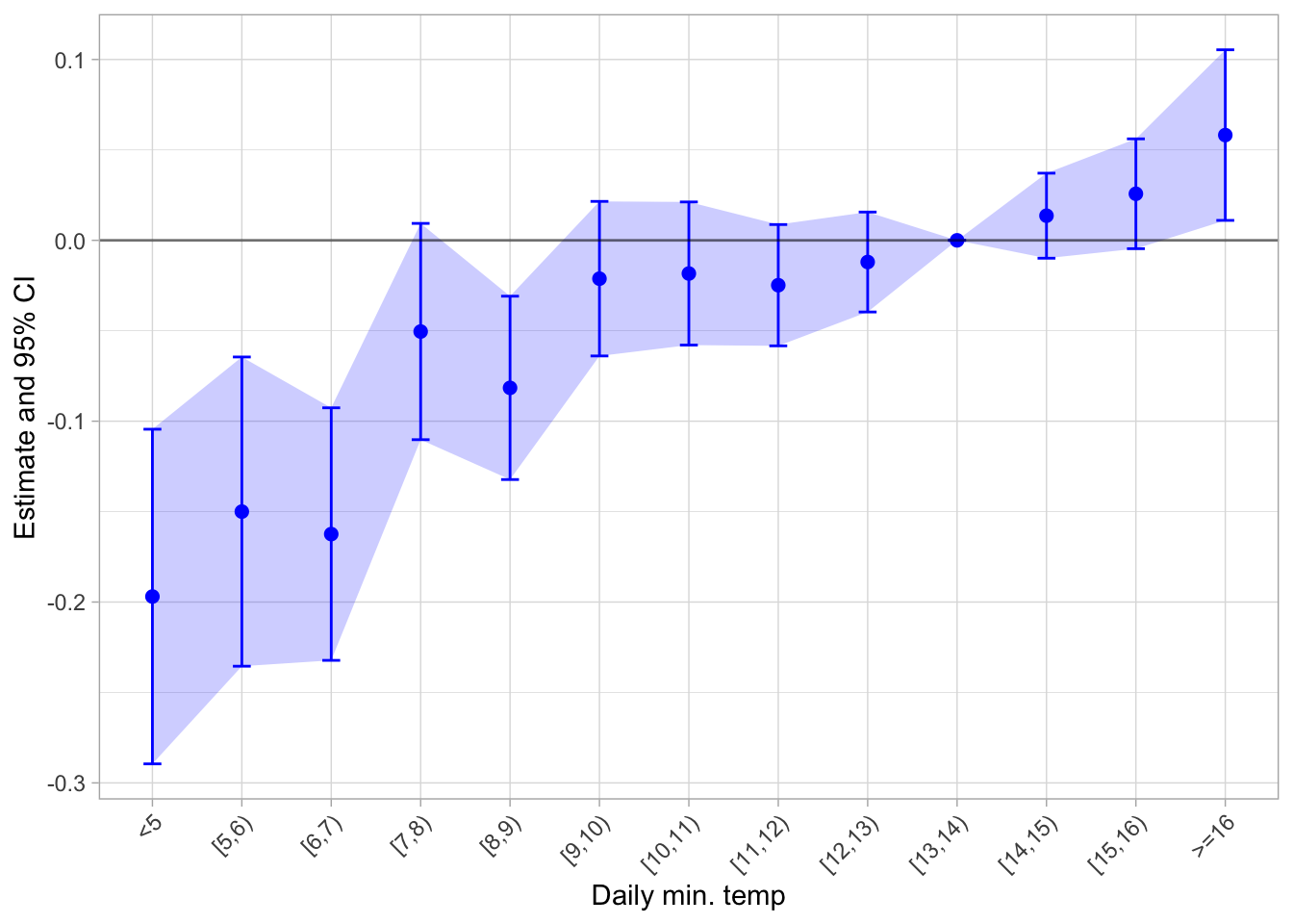
<- data %>% mutate (bins_tmin_one = create_dynamic_bins (tmin, width = 1 , 0.01 )) %>% fepois (reports_dv ~ i (bins_tmin_one, ref = "[13" ) | + rh_quintile + wsp_quintile + + year^ month + day_of_week + day_of_year,cluster = ~ ageb)
Plot and save as reg_bins_reports_tmin_1C.png
Reports with bins_midnight_temperature
I extract the midnight temperature from the hourly data. It is simply the first of the list of the 24 hourly measures.
<- data %>% left_join (read_rds (here (".." , "output" , "temporary_data" ,"tmp_hourly_ageb.rds" ))%>% mutate (midnight_temp = map_dbl (tmp_hourly, ~ .x[1 ]))
Run the reg:
<- data %>% mutate (bins_midnight_temp = create_dynamic_bins (midnight_temp, width = 1 , 0.01 )) %>% fepois (reports_dv ~ i (bins_midnight_temp, ref = "[13" ) | + rh_quintile + wsp_quintile + + year^ month + day_of_week + day_of_year,cluster = ~ ageb)
Plot and save as reg_bins_reports_midnight_temp.png
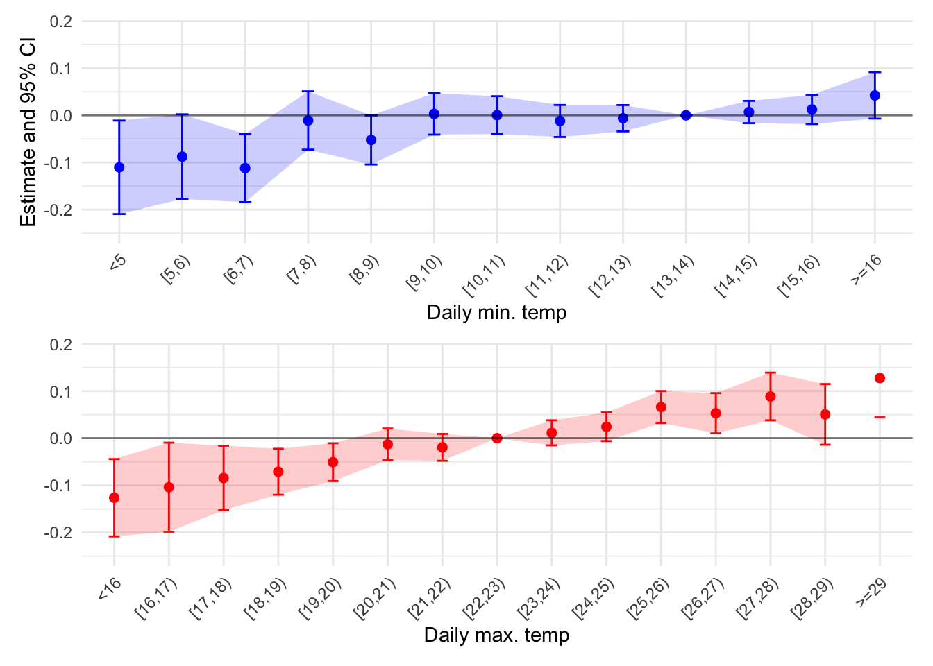
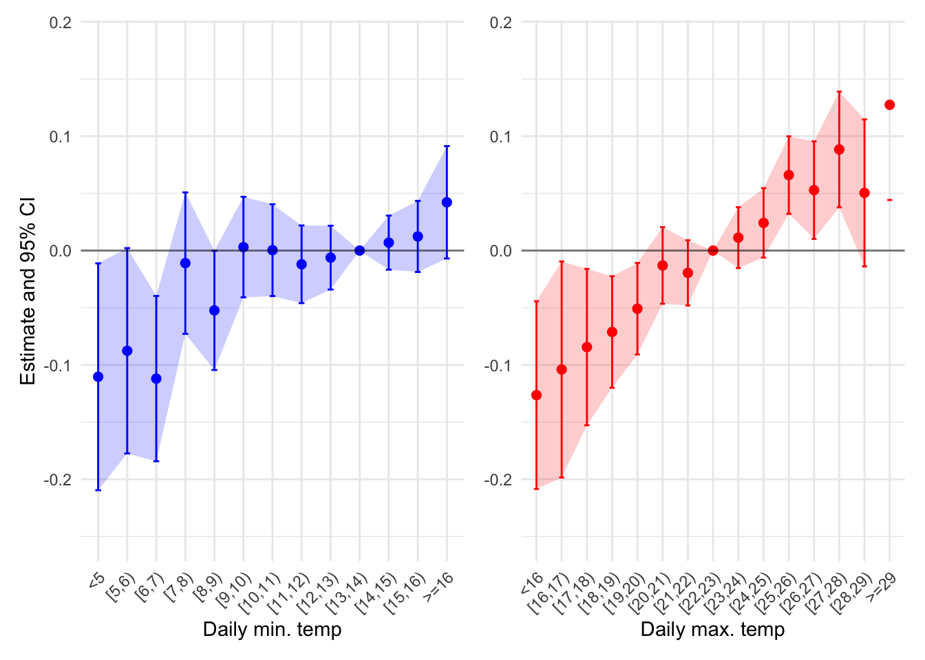
Reports with bins_tmin_one and bins_tmax_one estimated jointly
<- data %>% mutate (bins_tmin_one = create_dynamic_bins (tmin, width = 1 , 0.01 ),bins_tmax_one = create_dynamic_bins (tmax, width = 1 , 0.01 )) %>% fepois (reports_dv ~ i (bins_tmin_one, ref = "[13" ) + i (bins_tmax_one, ref = "[22" ) | + rh_quintile + wsp_quintile + + year^ month + day_of_week + day_of_year,cluster = ~ ageb)
Plot and save as reg_bins_reports_tmin_tmax_jointly.png and the horizontal version as reg_bins_reports_tmin_tmax_jointly_horizontal.png
Rendered on: 2025-07-27 01:41:43
Total render time: 1198.159 sec elapsed